TL;DR Learn how to create a Deep Convolutional Neural Network in TensorFlow.js and use it to classify images of Aliens and Predators

Staying alone in the corner, you and your motion detector. Total silence. Then you hear an unwanted beep and see a dot. 100 feet. 90 feet. You prepare yourself. This place is very dark, you think. You see something in the distance. Another beep - 20 feet. 10 feet. The thing is much more recognizable now, but what is it?

Here’s what you’ll learn:

• Load images from remote URLs in the browser
• Transform (turn to greyscale, resize and rescale) image pixel data into Tensors
• Build a simple Deep Convolutional Neural Network from scratch using TensorFlow.js
• Visualize filters (what the network learns) of convolutional layers

Let’s build a model that can distinguish between an Alien and a Predator!

Run the complete source code for this tutorial right in your browser:

Source code on GitHub

Data

Our dataset Alien vs. Predator images comes from Kaggle. Each class (alien and predator) contains 247 training images and 100 validation images. The images are JPG files with a size of around 250x250 pixels. Let’s use those to build a Neural Network that can classify them!

Convolutional Neural Networks

Building models that understand the real-world from raw image data has been a dream for many computer scientists. In recent years, this dream has been somewhat achieved.

Using traditional Machine Learning models for computer vision requires a manual definition of features. Convolutional Neural Networks allow for automation of this step. Those features are learned during the training from the raw image data.

Computers store images in width x height x 3 (or 4) tensors. The last dimension represents the colors (Red Green Blue) and a possible alpha channel. This poses a challenge for regular Neural Networks - every pixel (and color data) will be stored as a neuron. Some of the “getting started” image datasets are ok. CIFAR-10 has images of 32x32x3 = 3072 neurons. But we all know that images in the wild are huge!

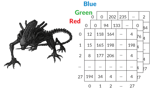
Convolutional Neural Networks (CNNs/ConvNets) take advantage of the two-dimensional image data. Still, they can be used with other types of data. CNNs consists of Convolutional, Pooling and Fully-Connected (regular) layers.

Convolutional layers have neurons arranged in 3 dimensions: width, height, depth. The parameters (those who we try to learn during training) consist of a set of learnable filters. Every filter covers a small area (width x height) but extends through the full depth.

During training, we slide each filter across the image`s height and weight and compute dot products between the filter and input.

One common way to design a Convolutional Neural Network for classification or regression is:

• Input Layer - holds the raw pixel values of the image
• Conv Layer - computes the dot product between filters and input data
• Pool Layer - downsamples the width and height of the input
• Fully-Connected Layer - delivers the predictions, based on the task at hand (classification or regression)

Classifying Aliens and Predators

We’ll load the image data from GitHub, do some preprocessing and train a CNN model with it.

Let’s look at an example image of an Alien:

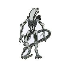
And a Predator:

One thing to note from these examples is that the type of images can be quite different. Let’s see if the model we’re going to build can handle that.

Data preprocessing

We’ll use the image-pixels package to load pixel data for our images:

1const loadImages = async urls => {
2  const imageData = await pixels.all(urls, { clip: [0, 0, 192, 192] })
3  return imageData.map(d =>
4    rescaleImage(resizeImage(toGreyScale(tf.browser.fromPixels(d))))
5  )
6}

We use the clip option to turn each image into 192x192 square. We convert each image into a Tensor using tf.browser.fromPixels, turn into greyscale, resize it and rescale:

1const toGreyScale = image => image.mean(2).expandDims(2)

To turn an image with color into greyscale we just take the mean from the values in the color channels.

1const TENSOR_IMAGE_SIZE = 28
2
3const resizeImage = image =>
4  tf.image.resizeBilinear(image, [TENSOR_IMAGE_SIZE, TENSOR_IMAGE_SIZE])

The resizing is done by tf.image.resizeBilinear and converts the image to a 28x28x3 Tensor.

1const rescaleImage = image => {
2  const expandedImage = image.expandDims(0)
3
4  return expandedImage.toFloat().div(tf.scalar(127)).sub(tf.scalar(1))
5}

Each pixel across each color channel has a value in the range of 0-255. We convert that to a range of -1 to 1 and add a dimension to our image Tensor.

Let’s load the images:

1const trainAlienImages = await loadImages(trainAlienImagePaths)
2const trainPredatorImages = await loadImages(trainPredatorImagePaths)
3
4const testAlienImages = await loadImages(validAlienImagePaths)
5const testPredatorImages = await loadImages(validPredatorImagePaths)

And prepare the training and test data (features and labels):

1const trainAlienTensors = tf.concat(trainAlienImages)
2
3const trainPredatorTensors = tf.concat(trainPredatorImages)
4
5const trainAlienLabels = tf.tensor1d(
6  _.times(TRAIN_IMAGES_PER_CLASS, _.constant(0)),
7  "int32"
8)
9
10const trainPredatorLabels = tf.tensor1d(
11  _.times(TRAIN_IMAGES_PER_CLASS, _.constant(1)),
12  "int32"
13)
14
15const testAlienTensors = tf.concat(testAlienImages)
16
17const testPredatorTensors = tf.concat(testPredatorImages)
18
19const testAlienLabels = tf.tensor1d(
20  _.times(VALID_IMAGES_PER_CLASS, _.constant(0)),
21  "int32"
22)
23
24const testPredatorLabels = tf.tensor1d(
25  _.times(VALID_IMAGES_PER_CLASS, _.constant(1)),
26  "int32"
27)
28
29const xTrain = tf.concat([trainAlienTensors, trainPredatorTensors])
30
31const yTrain = tf.concat([trainAlienLabels, trainPredatorLabels])
32
33const xTest = tf.concat([testAlienTensors, testPredatorTensors])
34
35const yTest = tf.concat([testAlienLabels, testPredatorLabels])

Note that we preserve the order of the training data, so we need to shuffle it later.

Building a Deep Convolutional Neural Network

Let’s have a look at how to build our CNN model:

1const { conv2d, maxPooling2d, flatten, dense } = tf.layers
2
3const model = tf.sequential()
4
5model.add(
6  conv2d({
7    name: "first-conv-layer",
8    inputShape: [TENSOR_IMAGE_SIZE, TENSOR_IMAGE_SIZE, 1],
9    kernelSize: 5,
10    filters: 8,
11    strides: 1,
12    activation: "relu",
13    kernelInitializer: "varianceScaling",
14  })
15)
16model.add(maxPooling2d({ poolSize: 2, strides: 2 }))
17
18model.add(
19  conv2d({
20    name: "second-conv-layer",
21    kernelSize: 5,
22    filters: 16,
23    strides: 1,
24    activation: "relu",
25    kernelInitializer: "varianceScaling",
26  })
27)
28model.add(maxPooling2d({ poolSize: 2, strides: 2 }))
29
30model.add(flatten())
31
32model.add(
33  dense({
34    units: 1,
35    kernelInitializer: "varianceScaling",
36    activation: "sigmoid",
37  })
38)
39
40model.compile({
41  optimizer: tf.train.adam(0.0001),
42  loss: "binaryCrossentropy",
43  metrics: ["accuracy"],
44})

We’re stacking two pairs of convolutional and max pooling layers. Each convolutional layer applies to 5x5 patches (kernelSize). Our downsizing operation reduces the size of the input by 2 (poolSize) and moves the application window by 2 pixels (right and down).

After computing all convolutions, we’re flattening the input (converting it to a single dimension) using tf.layers.flatten(). The output layer has a single neuron and sigmoid activation function. We use Adam optimizer and binary cross-entropy loss function.

All neurons are initialized (kernelInitializer) using varianceScaling.

Let’s have a look at the filters at the first convolutional layer before our model has seen the data (using the first 5 Alien and Predator images from the test set):

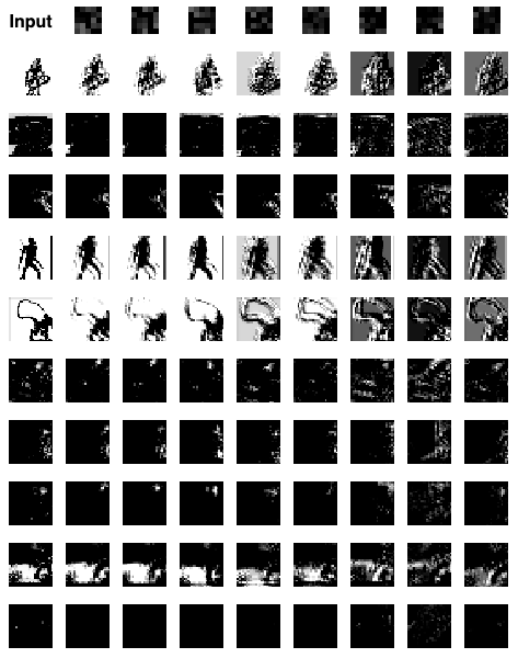
Looks like nothing is looking important to the untrained first layer. Let’s have a look at the second one:

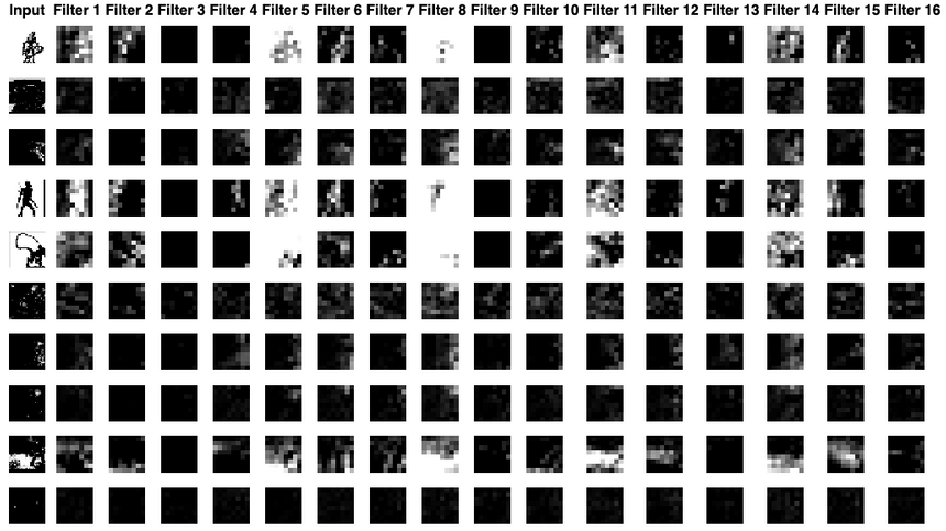
The same thing, the only difference is the size of the patches is much smaller. Let’s train our model and have another look at those filters.

Training

Training a CNN is not any different from a regular Deep Neural Network using TensorFlow.js. Let’s get to it:

1const lossContainer = document.getElementById("loss-cont")
2
3await model.fit(xTrain, yTrain, {
4  batchSize: 32,
5  validationSplit: 0.1,
6  shuffle: true,
7  epochs: 150,
8  callbacks: tfvis.show.fitCallbacks(
9    lossContainer,
10    ["loss", "val_loss", "acc", "val_acc"],
11    {
12      callbacks: ["onEpochEnd"],
13    }
14  ),
15})

Note that we shuffle the data, before training and using 10% of it for validation.

We have two perfectly balanced (equal number of examples) classes of images. We would expect that a dummy (random) model would predict with an accuracy of about 50%. How did we do?

Our model plateaus at around 62% accuracy which is not great, but we don’t have a particularly large dataset. Let’s dive a bit deeper into the performance.

Evaluation

Let’s see how well we predict each class using the confusion matrix:

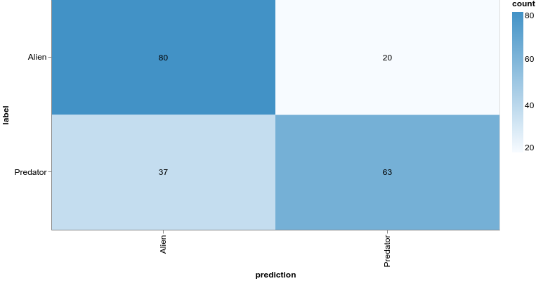
Looks like our model is doing better at “understanding” what an Alien is compared to a Predator. It is also biased towards predicting anything is an Alien.

What filters did our model learn in the first convolutional layer?

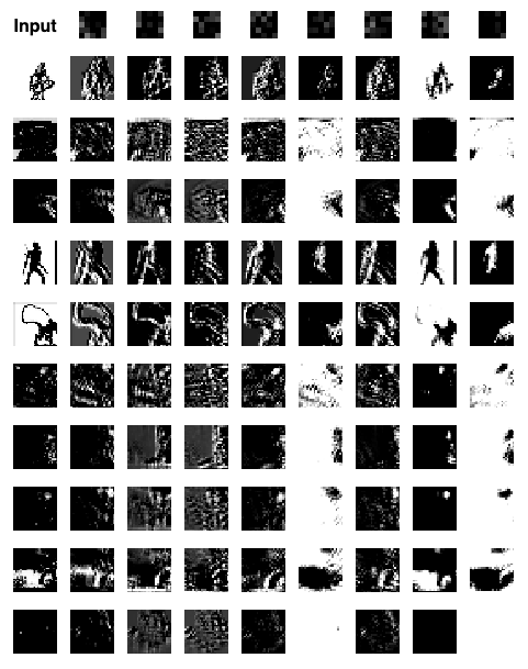
You can see that the visualization of the filters contains much fuzzier edges. We can see the same thing happening in the second layer:

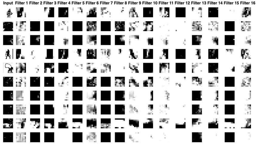
One interesting observation from this layer is the fact that most of the filters now contain highly contrasting patches. Seems like our model did learn something.

Conclusion

You just built your first Convolutional Neural Network model and can now use it to predict whether an image contains an Alien or a Predator. You also learned how to:

• Load images from remote URLs in the browser
• Transform (turn to greyscale, resize and rescale) image pixel data into Tensors
• Build a simple Deep Convolutional Neural Network from scratch using TensorFlow.js
• Visualize filters (what the network learns) of convolutional layers

The methods and techniques for building our model are very general and can be used for both classification and regression tasks when using raw image data. Try them on your own datasets!

Run the complete source code for this tutorial right in your browser:

Source code on GitHub

References

• Keras vs. PyTorch: Alien vs. Predator recognition with transfer learning

• Very Deep Convolutional Networks for Text Classification

• CS231n Convolutional Neural Networks