TL;DR Detect anomalies in S&P 500 daily closing price. Build LSTM Autoencoder Neural Net for anomaly detection using Keras and TensorFlow 2.

This guide will show you how to build an Anomaly Detection model for Time Series data. You’ll learn how to use LSTMs and Autoencoders in Keras and TensorFlow 2. We’ll use the model to find anomalies in S&P 500 daily closing prices.

This is the plan:

• Anomaly Detection
• LSTM Autoencoders
• S&P 500 Index Data
• LSTM Autoencoder in Keras
• Finding Anomalies

Run the complete notebook in your browser

The complete project on GitHub

Anomaly Detection

Anomaly detection refers to the task of finding/identifying rare events/data points. Some applications include - bank fraud detection, tumor detection in medical imaging, and errors in written text.

A lot of supervised and unsupervised approaches to anomaly detection has been proposed. Some of the approaches include - One-class SVMs, Bayesian Networks, Cluster analysis, and (of course) Neural Networks.

We will use an LSTM Autoencoder Neural Network to detect/predict anomalies (sudden price changes) in the S&P 500 index.

LSTM Autoencoders

Autoencoders Neural Networks try to learn data representation of its input. So the input of the Autoencoder is the same as the output? Not quite. Usually, we want to learn an efficient encoding that uses fewer parameters/memory.

The encoding should allow for output similar to the original input. In a sense, we’re forcing the model to learn the most important features of the data using as few parameters as possible.

Anomaly Detection with Autoencoders

Here are the basic steps to Anomaly Detection using an Autoencoder:

1. Train an Autoencoder on normal data (no anomalies)
2. Take a new data point and try to reconstruct it using the Autoencoder
3. If the error (reconstruction error) for the new data point is above some threshold, we label the example as an anomaly

Good, but is this useful for Time Series Data? Yes, we need to take into account the temporal properties of the data. Luckily, LSTMs can help us with that.

S&P 500 Index Data

Our data is the daily closing prices for the S&P 500 index from 1986 to 2018.

The S&P 500, or just the S&P, is a stock market index that measures the stock performance of 500 large companies listed on stock exchanges in the United States. It is one of the most commonly followed equity indices, and many consider it to be one of the best representations of the U.S. stock market. -Wikipedia

It is provided by Patrick David and hosted on Kaggle. The data contains only two columns/features - the date and the closing price. Let’s download and load into a Data Frame:

1!gdown --id 10vdMg_RazoIatwrT7azKFX4P02OebU76 --output spx.csv

1df = pd.read_csv('spx.csv', parse_dates=['date'], index_col='date')

Let’s have a look at the daily close price:

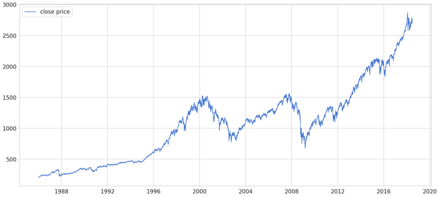
That trend (last 8 or so years) looks really juicy. You might want to board the train. When should you buy or sell? How early can you “catch” sudden changes/anomalies?

Preprocessing

We’ll use 95% of the data and train our model on it:

1train_size = int(len(df) * 0.95)
2test_size = len(df) - train_size
3train, test = df.iloc[0:train_size], df.iloc[train_size:len(df)]
4print(train.shape, test.shape)

1(7782, 1) (410, 1)

Next, we’ll rescale the data using the training data and apply the same transformation to the test data:

1from sklearn.preprocessing import StandardScaler
2
3scaler = StandardScaler()
4scaler = scaler.fit(train[['close']])
5
6train['close'] = scaler.transform(train[['close']])
7test['close'] = scaler.transform(test[['close']])

Finally, we’ll split the data into subsequences. Here’s the little helper function for that:

1def create_dataset(X, y, time_steps=1):
2    Xs, ys = [], []
3    for i in range(len(X) - time_steps):
4        v = X.iloc[i:(i + time_steps)].values
5        Xs.append(v)
6        ys.append(y.iloc[i + time_steps])
7    return np.array(Xs), np.array(ys)

We’ll create sequences with 30 days worth of historical data:

1TIME_STEPS = 30
2
3# reshape to [samples, time_steps, n_features]
4
5X_train, y_train = create_dataset(
6  train[['close']],
7  train.close,
8  TIME_STEPS
9)
10
11X_test, y_test = create_dataset(
12  test[['close']],
13  test.close,
14  TIME_STEPS
15)
16
17print(X_train.shape)

1(7752, 30, 1)

The shape of the data looks correct. How can we make LSTM Autoencoder in Keras?

LSTM Autoencoder in Keras

Our Autoencoder should take a sequence as input and outputs a sequence of the same shape. Here’s how to build such a simple model in Keras:

1model = keras.Sequential()
2model.add(keras.layers.LSTM(
3    units=64,
4    input_shape=(X_train.shape[1], X_train.shape[2])
5))
6model.add(keras.layers.Dropout(rate=0.2))
7model.add(keras.layers.RepeatVector(n=X_train.shape[1]))
8model.add(keras.layers.LSTM(units=64, return_sequences=True))
9model.add(keras.layers.Dropout(rate=0.2))
10model.add(
11  keras.layers.TimeDistributed(
12    keras.layers.Dense(units=X_train.shape[2])
13  )
14)
15
16model.compile(loss='mae', optimizer='adam')

There are a couple of things that might be new to you in this model. The RepeatVector layer simply repeats the input n times. Adding return_sequences=True in LSTM layer makes it return the sequence.

Finally, the TimeDistributed layer creates a vector with a length of the number of outputs from the previous layer. Your first LSTM Autoencoder is ready for training.

Training the model is no different from a regular LSTM model:

1history = model.fit(
2    X_train, y_train,
3    epochs=10,
4    batch_size=32,
5    validation_split=0.1,
6    shuffle=False
7)

Evaluation

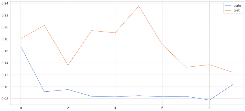
We’ve trained our model for 10 epochs with less than 8k examples. Here are the results:

Finding Anomalies

Still, we need to detect anomalies. Let’s start with calculating the Mean Absolute Error (MAE) on the training data:

1X_train_pred = model.predict(X_train)
2
3train_mae_loss = np.mean(np.abs(X_train_pred - X_train), axis=1)

Let’s have a look at the error:

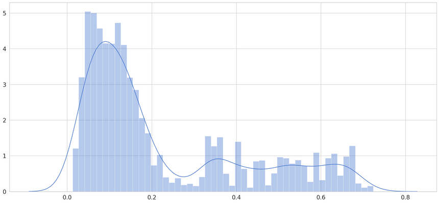
We’ll pick a threshold of 0.65, as not much of the loss is larger than that. When the error is larger than that, we’ll declare that example an anomaly:

1THRESHOLD = 0.65

Let’s calculate the MAE on the test data:

1X_test_pred = model.predict(X_test)
2
3test_mae_loss = np.mean(np.abs(X_test_pred - X_test), axis=1)

We’ll build a DataFrame containing the loss and the anomalies (values above the threshold):

1test_score_df = pd.DataFrame(index=test[TIME_STEPS:].index)
2test_score_df['loss'] = test_mae_loss
3test_score_df['threshold'] = THRESHOLD
4test_score_df['anomaly'] = test_score_df.loss > test_score_df.threshold
5test_score_df['close'] = test[TIME_STEPS:].close

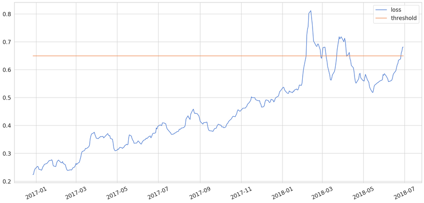
Looks like we’re thresholding extreme values quite well. Let’s create a DataFrame using only those:

1anomalies = test_score_df[test_score_df.anomaly == True]

Finally, let’s look at the anomalies found in the testing data:

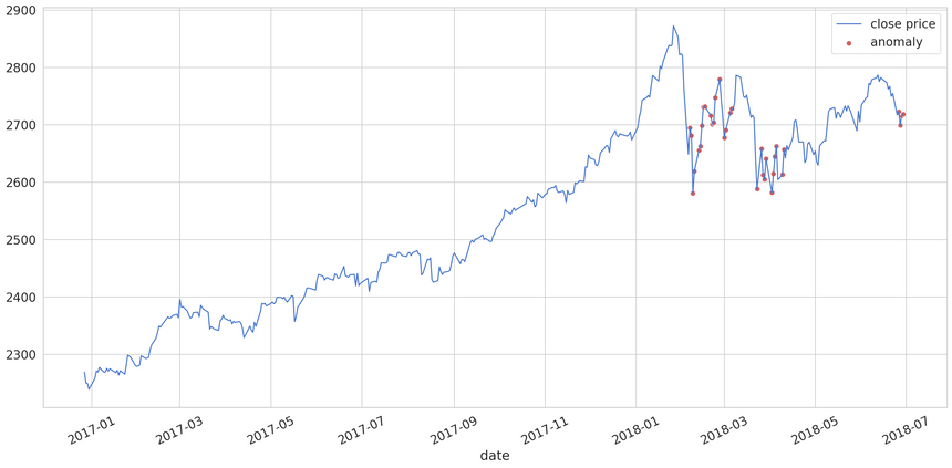
You should have a thorough look at the chart. The red dots (anomalies) are covering most of the points with abrupt changes to the closing price. You can play around with the threshold and try to get even better results.

Conclusion

You just combined two powerful concepts in Deep Learning - LSTMs and Autoencoders. The result is a model that can find anomalies in S&P 500 closing price data. You can try to tune the model and/or the threshold to get even better results.

Here’s a recap of what you did:

• Anomaly Detection
• LSTM Autoencoders
• S&P 500 Index Data
• LSTM Autoencoder in Keras
• Finding Anomalies

Run the complete notebook in your browser

The complete project on GitHub

Can you apply the model to your dataset? What results did you get?

References

• TensorFlow - Time series forecasting
• Understanding LSTM Networks
• Step-by-step understanding LSTM Autoencoder layers
• S&P500 Daily Prices 1986 - 2018