TL;DR Build a Decision Tree regression model using Python from scratch. Compare the performance of your model with that of a Scikit-learn model. The Decision Tree is used to predict house sale prices and send the results to Kaggle.

I am sorry, you might be losing sleep. Deep down you know your Linear Regression model ain’t gonna cut it. That housing market domination is still further down the road.

Can we improve that, can we have a model that makes better predictions?

Complete source code notebook on Google Colaboratory

The Data

Once again, we’re going to use the Kaggle data: “House Prices: Advanced Regression Techniques”. It contains 1460 training data points and 80 features that might help us predict the selling price of a house.

Decision Trees

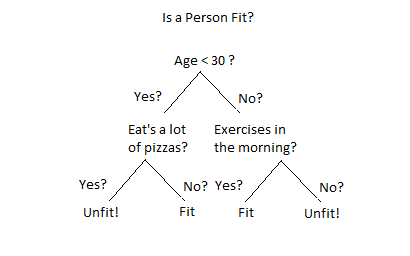
Decision tree models build structures like this:

source: https://www.xoriant.com

The algorithms for building trees breaks down a data set into smaller and smaller subsets while an associated decision tree is incrementally developed. The final result is a tree with decision nodes and leaf nodes. A decision node has two or more branches. Leaf node represents a classification or decision (used for regression). The topmost decision node in a tree which corresponds to the best predictor (most important feature) is called a root node.

Decision trees can handle both categorical and numerical data. They are used for classification and regression problems. They can handle missing data pretty well, too!

Data Preprocessing

We’re going to use the same data we used with the Linear Regression model. However, we’re not going to do any scaling, just because we’re lazy (or it is not needed):

1X = df_train[['OverallQual', 'GrLivArea', 'GarageCars']]
2y = df_train['SalePrice']

Cost function

We’re going to use a new cost function — Root Mean Square Error (RMSE). It is the standard deviation of how far from the regression line data points are. In other words, it tells you how concentrated the data is around the line of best fit.

RMSE is given by the formula:

We’ve already implemented MSE in previous parts, so we’re going to import an implementation here, in the name of readability (or holy laziness?):

1from sklearn.metrics import mean_squared_error
2from math import sqrt
3
4def rmse(h, y):
5  return sqrt(mean_squared_error(h, y))

Using a prebuild Decision Tree model

Let use Decision Tree regressor from the scikit-learn library to get a quick feel of the model:

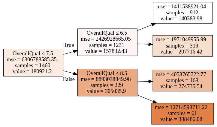
1from sklearn.ensemble import RandomForestRegressor
2
3reg = RandomForestRegressor(
4  n_estimators=1,
5  max_depth=2,
6  bootstrap=False,
7  random_state=RANDOM_SEED
8)
9reg.fit(X, y)

We are using RandomForestRegressor with 1 estimator, which basically means we’re using a Decision Tree model. Here is the tree structure of our model:

You should receive the exact same model (if you’re running the code) since we are setting the random state. How many features did the model use?

Now that this model is ready to be used let’s evaluate its R² score:

1preds = reg.predict(X)
2metrics.r2_score(y, preds)

10.6336246655552089

The $R^2$ statistic gives us information about the goodness of fit of the model. A score of 1 indicates perfect fit. Let’s have a look at the RMSE:

148069.23940764968

Building your own Decision Tree

1class DecisionTreeRegressor:
2
3  def fit(self, X, y, min_leaf = 5):
4    self.dtree = Node(X, y, np.array(np.arange(len(y))), min_leaf)
5    return self
6
7  def predict(self, X):
8    return self.dtree.predict(X.values)

Let’s start implementing our Node helper class:

1class Node:
2
3    def __init__(self, x, y, idxs, min_leaf=5):
4        self.x = x
5        self.y = y
6        self.idxs = idxs
7        self.min_leaf = min_leaf
8        self.row_count = len(idxs)
9        self.col_count = x.shape[1]
10        self.val = np.mean(y[idxs])
11        self.score = float('inf')
12        self.find_varsplit()

Trees are recursive data structures and we’re going to take full advantage of that. Our Node class represents one decision point in our model. Each division within the model has 2 possible outcomes for finding a solution — go to the left or go to the right. That decision point also divides our data into two sets.

The property idxs stores indexes of the subset of the data that this Node is working with.

The decision (prediction) is based on the value that Node holds. To make that prediction we’re just going to take the average of the data of the dependent variable for this Node.

The method find_varsplit finds where should we split the data. Let’s have a look at it:

1def find_varsplit(self):
2    for c in range(self.col_count): self.find_better_split(c)
3    if self.is_leaf: return
4    x = self.split_col
5    lhs = np.nonzero(x <= self.split)[0]
6    rhs = np.nonzero(x > self.split)[0]
7    self.lhs = Node(self.x, self.y, self.idxs[lhs], self.min_leaf)
8    self.rhs = Node(self.x, self.y, self.idxs[rhs], self.min_leaf)

First, we try to find a better feature to split on. If no such feature is found (we’re at a leaf node) we do nothing. Then we use the split value found by find_better_split, create the data for the left and right nodes and create each one using a subset of the data.

Here are the split_col and is_leaf implementations:

1@property
2def split_col(self): return self.x.values[self.idxs,self.var_idx]
3
4@property
5def is_leaf(self): return self.score == float('inf')

It is time to implement the workhorse of our algorithm find_better_split method:

1def find_better_split(self, var_idx):
2    x = self.x.values[self.idxs, var_idx]
3
4    for r in range(self.row_count):
5        lhs = x <= x[r]
6        rhs = x > x[r]
7        if rhs.sum() < self.min_leaf or lhs.sum() < self.min_leaf: continue
8
9        curr_score = self.find_score(lhs, rhs)
10        if curr_score < self.score:
11            self.var_idx = var_idx
12            self.score = curr_score
13            self.split = x[r]
14
15def find_score(self, lhs, rhs):
16    y = self.y[self.idxs]
17    lhs_std = y[lhs].std()
18    rhs_std = y[rhs].std()
19    return lhs_std * lhs.sum() + rhs_std * rhs.sum()

We are trying to split on each data point and let the best split wins.

We’re going to create our split such that it has as low standard deviation as possible. We find the split that minimizes the weighted averages of the standard deviations which is equivalent to minimizing RMSE.

If we find a better split we store the following information: index of the variable, split score and value of the split.

The score is a metric that tells us how effective the split was (note that leaf nodes do not have scores, so it will be infinity). The method find_score calculates a weighted average of the data. If the score is lower than the previous we have a better split. Note that the score is initially set to infinity -> only leaf nodes and really shallow trees (and Thanos) have a score of infinity.

Finally, let’s look at how we use all this to make predictions:

1def predict(self, x):
2    return np.array([self.predict_row(xi) for xi in x])
3
4def predict_row(self, xi):
5    if self.is_leaf: return self.val
6    node = self.lhs if xi[self.var_idx] <= self.split else self.rhs
7    return node.predict_row(xi)

Once again, we’re exploiting the recursive nature of life. Starting at the tree root, predict_row checks if we need to go left or right node based on the split value we found. The recursion ends once we hit a leaf node. At that point, the answer/prediction is stored in the val property.

Here is the complete source of our Node class:

1class Node:
2
3    def __init__(self, x, y, idxs, min_leaf=5):
4        self.x = x
5        self.y = y
6        self.idxs = idxs
7        self.min_leaf = min_leaf
8        self.row_count = len(idxs)
9        self.col_count = x.shape[1]
10        self.val = np.mean(y[idxs])
11        self.score = float('inf')
12        self.find_varsplit()
13
14    def find_varsplit(self):
15        for c in range(self.col_count): self.find_better_split(c)
16        if self.is_leaf: return
17        x = self.split_col
18        lhs = np.nonzero(x <= self.split)[0]
19        rhs = np.nonzero(x > self.split)[0]
20        self.lhs = Node(self.x, self.y, self.idxs[lhs], self.min_leaf)
21        self.rhs = Node(self.x, self.y, self.idxs[rhs], self.min_leaf)
22
23    def find_better_split(self, var_idx):
24
25        x = self.x.values[self.idxs, var_idx]
26
27        for r in range(self.row_count):
28            lhs = x <= x[r]
29            rhs = x > x[r]
30            if rhs.sum() < self.min_leaf or lhs.sum() < self.min_leaf: continue
31
32            curr_score = self.find_score(lhs, rhs)
33            if curr_score < self.score:
34                self.var_idx = var_idx
35                self.score = curr_score
36                self.split = x[r]
37
38    def find_score(self, lhs, rhs):
39        y = self.y[self.idxs]
40        lhs_std = y[lhs].std()
41        rhs_std = y[rhs].std()
42        return lhs_std * lhs.sum() + rhs_std * rhs.sum()
43
44    @property
45    def split_col(self): return self.x.values[self.idxs,self.var_idx]
46
47    @property
48    def is_leaf(self): return self.score == float('inf')
49
50    def predict(self, x):
51        return np.array([self.predict_row(xi) for xi in x])
52
53    def predict_row(self, xi):
54        if self.is_leaf: return self.val
55        node = self.lhs if xi[self.var_idx] <= self.split else self.rhs
56        return node.predict_row(xi)

Evaluation

Let’s check how your Decision Tree regressor does on the training data:

1regressor = DecisionTreeRegressor().fit(X, y)
2preds = regressor.predict(X)

Here is the $R^2$ score:

10.8504381072711565

Our scikit-learn model gave us a score of 0.6336246655552089

The RMSE score is:

130712.460628635836

The scikit-learn regressor gave us 48069.23940764968

Looks like your model is doing pretty good, eh? Let’s make a prediction on the test data and send it to Kaggle.

Sending your predictions to Kaggle

Let make our predictions and format the data as requested on Kaggle:

1X_test = df_test[['OverallQual', 'GrLivArea', 'GarageCars']]
2pred_test = regressor.predict(X_test)
3
4submission = pd.DataFrame({'Id': df_test.Id, 'SalePrice': pred_test})
5submission.to_csv('submission.csv', index=False)

Feel free to submit your csv file to Kaggle. Also, how can you improve?

Complete source code notebook on Google Colaboratory

Conclusion

Give yourself a treat, you just implemented a Decision Tree regressor!

Would it be possible to implement Random Forest regressor on top of your model? How that affects your Kaggle scores?

In the next part, you’re gonna do some unsupervised learning with k means!

Acknowledgments

The source code presented in this part is heavily inspired by the excellent course of fast.ai — Introduction to Machine Learning for Coders