TL;DR Build a simple Neural Network model in TensorFlow.js to make a laptop buying decision. Learn why Neural Networks need activation functions and how should you initialize their weights.

It is in the middle night, and you’re dreaming some rather alarming dreams with a smile on your face. Suddenly, your phone starts ringing, rather internationally. You pick up, half-asleep, and listen to something bizarre.

A friend of yours is calling, from the other side of our planet, asking for help in picking a laptop. After all, it is Black Friday!

You’re a bit dazzled by the fact that this is the first time you hear from your friend in 5 years. Still, you’re a good person and agree to help out. Maybe it is time to put your TensorFlow.js skills into practice?

How about you build a model to help out your friend so you can get back to sleep? You heard that Neural Networks are pretty hot right now. It is 3 in the morning, there isn’t much need for persuasion in your mind. You’ll use a Neural Network for this one!

Run the complete source code for this tutorial right in your browser:

Neural Networks

What is a Neural Network? In a classical cliff-hanger fashion, we’ll start far away from answering this question.

Neural Networks were around for a while (since 1950s)? Why did they become popular just recently (last 5-10 years)? First introduced by Warren McCulloch and Walter Pitts in A logical calculus of the ideas immanent in nervous activity Neural Networks were really popular until the mid-1980s when Support Vector Machines and other methods overtook the community.

The Universal approximation theorem states that a Neural Networks can approximate any function (under some mild assumptions), even with a single hidden layer (more on that later). One of the first proves was done by George Cybenko in 1989 for sigmoid activation functions (will have a look at those in a bit).

More recently, more and more advances in the field of Deep Learning made Neural Networks a hot topic again. Why? We’ll discuss that a bit later. First, let’s start with the basics!

The Perceptron

The original model, intended to model how the human brain processed visual data and learned to recognize objects, was susggested by Frank Rosenblatt in the 1950s. The Perceptron takes one or more binary inputs $x_1, x_2, \ldots, x_n$ and produces a binary output:

To compute the output you have to:

• have weights $w_1, w_2, \ldots, w_n$ expressing the importance of the respective input
• the binary output (0 or 1) is determined by whether the weighted sum $\sum_j w_j x_j$ is greater or lower than some threshold

Let’s have a look at an example. Imagine you need to decide whether or not you need a new laptop. The most important features are its color and size (that’s what she said). So, you have two inputs:

1. is it pink?
2. is it small (gotcha)?

You can represent these factors with binary variables $x_{pink}$, $x_{small}$ and assign weights/importance $w_{pink}$, $w_{small}$ to each one. Depending on the importance you assign to each factor, you can get different models.

We can simplify the Perceptron even further. We can rewrite $\sum_j w_j x_j$ as a dot product of two vectors $w \cdot x$. Next, we’ll introduce the Perceptron’s bias, $b = -{\text{threshold}}$. Using it, we can rewrite the model as:

The bias is a measure of how easy it is for a perceptron to output 1 (to fire). Large positive bias makes outputting 1 easy, while a large negative bias makes it difficult.

Let’s build the Perceptron model using TensorFlow.js:

1const perceptron = ({ x, w, bias }) => {
2  const product = tf.dot(x, w).dataSync()[0]
3  return product + bias < 0 ? 0 : 1
4}

An offer for a laptop comes around. It is not pink, but it is small $x = \begin{bmatrix}0\\1\end{bmatrix}$. You’re biased towards not buying a laptop because you’re broke. You can encode that with a negative bias. You’re one of the brainier users, and you put more emphasis on size, rather than color $w = \begin{bmatrix}0.5\\0.9\end{bmatrix}$:

1perceptron({
2  x: [0, 1],
3  w: [0.5, 0.9],
4  bias: -0.5,
5})

11

Yes, you have to buy that laptop!

Sigmoid neuron

To make learning from data possible, we want the weights of our model to change only by a small amount when presented with an example. That is, each example should cause a small change in the output.

That way, one can continuously adjust the weights while presenting new data and not worrying that a single example will wipe out everything the model has learned so far.

The Perceptron is not an ideal for that purpose since small changes in the inputs are propagated linearly to the output. We can overcome this using a sigmoid neuron.

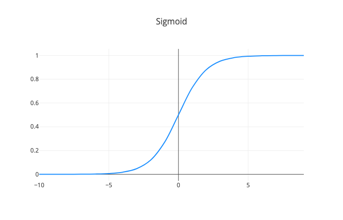
The sigmoid neuron has inputs $x_1, x_2, \ldots, x_n$ that can be values between 0 and 1. The output is given by $\sigma(w \cdot x + b)$ where $\sigma$ is the sigmoid function, defined by:

Let’s have a look at it using TensorFlow.js and Plotly:

1const xs = [...Array(20).keys()].map(x => x - 10)
2const ys = tf.sigmoid(xs).dataSync()
3
4renderActivationFunction(xs, ys, "Sigmoid", "sigmoid-cont")

Using the weights and inputs we get:

Let’s dive deeper into the sigmoid neuron and understand the similarities with the Perceptron:

• Suppose that $z$ is a large positive number. Then $e^{-z} \approx 0$ and $\sigma(z) \approx 1$.
• Suppose that $z$ is a large negative number. Then $e^{-z} \rightarrow \infty$ and $\sigma(z) \approx 0$.
• When $z$ is somewhat modest, we observe a significant difference compared to the Perceptron.

Let’s build the sigmoid neuron model using TensorFlow.js:

1const sigmoidPerceptron = ({ x, w, bias }) => {
2  const product = tf.dot(x, w).dataSync()[0]
3  return tf.sigmoid(product + bias).dataSync()[0]
4}

Another offer for a laptop comes around. This time you can specify the degree of how close the color is to pink and how small it is.

The color is somewhat pink, and the size is just about right $x = \begin{bmatrix}0.6\\0.9\end{bmatrix}$. The rest stays the same:

1sigmoidPerceptron({
2  x: [0.6, 0.9],
3  w: [0.5, 0.9],
4  bias: -0.5,
5})

10.6479407548904419

Yes, you still want to buy this laptop, but this model also outputs the confidence of its decision. Cool, right?

Architecting Neural Networks

A natural way to extend the models presented above is to group them in some way. One way to do that is to create layers of neurons. Here’s a simple Neural Network that can be used to make the decision of buying a laptop:

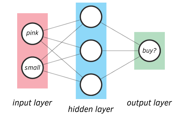
Neural Networks are a collection of neurons, connected in an acyclic graph. Outputs of some neurons are used as inputs to other neurons. They are organized into layers. Our example is composed of fully-connected layers (all neurons between two adjacent layers are connected), and it is a 2 layer Neural Network (we do not count the input layer). Neural Networks can make complex decisions thanks to combination of simple decisions made by the neurons that construct them.

Of course, the output layer contains the answer(s) you’re looking for. Let’s have a look at some of the ingredients that make training Neural Networks possible:

Activation functions

The Perceptron model is just a linear transformation. Stacking multiple such neurons on each other results in a vector product and a bias addition. Unfortunately, there are a lot of functions that can’t be estimated by a linear transformation.

The activation function makes it possible for the model to approximate non-linear functions (predict more complex phenomena). The good thing is, you’ve already met one activation function - the sigmoid:

One major disadvantage of the Sigmoid function is the is that it becomes really flat outside the [-3, +3] range. This leads to weights getting close to 0 - no learning is happening.

ReLU

ReLU, introduced in the context of Neural Networks in Rectified Linear Units Improve Restricted Boltzmann Machines, have a linear output at values greater than 0 and 0 otherwise.

Let’s have a look:

1const xs = [...Array(20).keys()].map(x => x - 10)
2const ys = tf.relu(xs).dataSync()
3
4renderActivationFunction(xs, ys, "ReLU", "relu-cont")

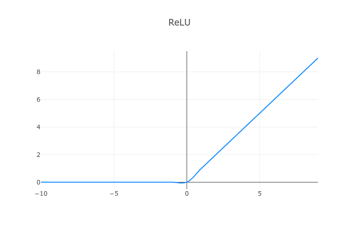
One disadvantage of ReLU is that negative values “die out” and stay at 0 - no learning.

Leaky ReLU

Leaky ReLU, introduced in Rectifier Nonlinearities Improve Neural Network Acoustic Models, solves the dead values introduced by ReLu:

1const xs = [...Array(20).keys()].map(x => x - 10)
2const ys = tf.leakyRelu(xs).dataSync()
3
4renderActivationFunction(xs, ys, "Leaky ReLU", "leaky-relu-cont")

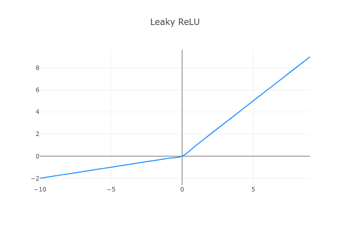
Note that negative values get scaled instead of zeroed out. Scaling is adjustable by a parameter in tf.leakyRelu().

Weight initialization

The process of teaching a Neural Network to make “reasonable” predictions involves adjusting the weights of the neurons multiple times. Those weights need to have initial values. How should you choose those?

The initialization process must take into account the algorithm we’re using to train our model. More often than not, that algorithm is Stochastic gradient descent (SGD). Its job is to do a search over possible parameters/weights and choose those that minimize the errors our model makes. Moreover, the algorithm heavily relies on randomness and a good starting point (given by the weights).

Same constant initialization

Imagine that we initialize the weights using the same constant (yes, including 0). Every neuron in the network will compute the same output, which results in the same weight/parameter update. We just defeated the purpose of having multiple neurons.

Too small/large value initialization

Let’s initialize the weights with a set of small values. Passing those values to the activation functions will decrease them exponentially, leaving every weight equally unimportant.

On the other hand, initializing with large values will lead to an exponential increase, making the weights equally unimportant again.

Random small number initialization

We can use a Normal distribution with a mean 0 and standard deviation 1 to initialize the weights with small random numbers.

Every neuron will compute different output, which leads to different parameter updates. Of course, multiple other ways exist. Check the TensorFlow.js Initializers

Should you buy the laptop?

Now that you know some Neural Network kung-fu, we can use TensorFlow.js to build a simple model and decide whether you should buy a given laptop.

Laptop data

Let’s say that for your friend, size is much more important than the degree of pinkness! You sit down and devise the following dataset:

1const X = tf.tensor2d([
2  // pink, small
3  [0.1, 0.1],
4  [0.3, 0.3],
5  [0.5, 0.6],
6  [0.4, 0.8],
7  [0.9, 0.1],
8  [0.75, 0.4],
9  [0.75, 0.9],
10  [0.6, 0.9],
11  [0.6, 0.75],
12])
13
14// 0 - no buy, 1 - buy
15const y = tf.tensor([0, 0, 1, 1, 0, 0, 1, 1, 1].map(y => oneHot(y, 2)))

Well done! You did well on incorporating your friend preferences.

Building the model

Recall the Neural Network we’re going to build:

Let’s translate it into a TensorFlow.js model:

1const model = tf.sequential()
2
3model.add(
4  tf.layers.dense({
5    inputShape: [2],
6    units: 3,
7    activation: "relu",
8  })
9)
10
11model.add(
12  tf.layers.dense({
13    units: 2,
14    activation: "softmax",
15  })
16)

We have a 2-layer network with an input layer containing 2 neurons, a hidden layer with 3 neurons and an output layer containing 2 neurons.

Note that we use ReLu activation function in the hidden layer and softmax for the output layer. We have 2 neurons in the output layer since we want to obtain how certain our Neural Network is in its buy/no-buy decision.

1model.compile({
2  optimizer: tf.train.adam(0.1),
3  loss: "binaryCrossentropy",
4  metrics: ["accuracy"],
5})

We’re using binary crossentropy to measure the quality of the current weights/parameters of our model by measuring how “good” the predictions are.

Our training algorithm, Stochastic gradient descent, is trying to find weights that minimize the loss function. For our example, we’re going to use the Adam optimizer.

Training

Now that our model is defined, we can use our training dataset to teach it about our friend preferences:

1await model.fit(X, y, {
2  shuffle: true,
3  epochs: 20,
4  callbacks: {
5    onEpochEnd: async (epoch, logs) => {
6      console.log("Epoch " + epoch)
7      console.log("Loss: " + logs.loss + " accuracy: " + logs.acc)
8    },
9  },
10})

We’re shuffling the data before training and log the progress after each epoch is complete:

1Epoch 1
2Loss: 0.703386664390564 accuracy: 0.5
3Epoch 2
4Loss: 0.6708164215087891 accuracy: 0.5555555820465088
5Epoch 3
6Loss: 0.6340110898017883 accuracy: 0.6666666865348816
7Epoch 4
8Loss: 0.6071969270706177 accuracy: 0.7777777910232544
9...
10Epoch 19
11Loss: 0.08228953927755356 accuracy: 1
12Epoch 20
13Loss: 0.06922533363103867 accuracy: 1

After 20 epochs or so seems like the model has learned the preferences of your friend.

Evaluation

You save the model and send it over to your friend. After connecting to your friend computer, you find somewhat appropriate laptop and encode the information into the model:

1const predProb = model.predict(tf.tensor2d([[0.1, 0.6]])).dataSync()

After waiting a few long milliseconds, you receive an answer:

10: 0.45
21: 0.55

The model agrees with you. It “thinks” that your friend should buy the laptop but it is not that certain about it. You did good!

Conclusion

Your friend seems happy with the results, and you’re thinking of making millions with your model by selling it as a browser extension. Either way, you learned a lot about:

• The Perceptron model
• Why activation functions are needed and which one to use
• How to initialize the weights of your Neural Network models
• Build a simple Neural Network to solve a (somewhat) real problem

Run the complete source code for this tutorial right in your browser:

Laying back on the comfy pillow, you start thinking. Could I’ve used Deep Learning for this?

References

Reducing Loss: Gradient Descent

Gradient descent and stochastic gradient descent from scratch

Initializing neural networks

Types of weight intializations

What if do not use any activation function in the neural network?