Build a taxi driving agent in a post-apocalyptic world using Reinforcement Learning | Machine Learning from Scratch (Part VIII)
— Machine Learning, Reinforcement Learning, MDP, Q-Learning, Self-driving — 8 min read
Share
TL;DR Build a simple MDP for self-driving taxi problem. Pick up passengers, avoid danger and drop them off at a specified location. Build an agent and solve the problem using Q-learning.
You wake up. It is a sunny day. Your partner is still asleep next to you. You take a minute to admire the beauty and even crack a smile.
Your stomach is rumbling, so you jump on your feet and look around. Jackpot! You’re looking at the leftovers of the anniversary dinner you two had last night. You take a minute to scratch some private spot of yours. Yep, what an amazing morning! You have 1/3 of a bean can, expired only 6 months ago. It is delicious!
Although you feel bad about not leaving any food for the one sleeping in your bed, you dress up and prepare for work. “What are you going to do? Not eat and work!?” - those thoughts don’t seem to help anymore. Time to hop in the car!
You try to reach Johny via the radio but no luck. Oh well, Jimmy is missing since last week, his twin brother might be too. Strange, you can’t remember the last time your eyes were feeling wet.
A lot has changed since the event. The streets are getting more dangerous every week, but people still need transportation. You receive a pickup request and have a look at the anomaly map. You accept hesitantly. Your map was updated 2 months ago.
You got the job done and got credit for a half can. That couple was really generous! That leaves time for tinkering with the idea of making self-driving taxis. You even got a name - SafeCab. You read a lot of about this crazy guy called Elon Nusk that was trying to build those fully autonomous vehicles right before the event occurred.
You start scratching your head. Is this possible or just a fantasy? After all, if you get this done, you might afford to eat every other day. Enter Reinforcement Learning.
Complete source code in Google Colaboratory Notebook
Reinforcement Learning
Reinforcement Learning (RL) is concerned with producing algorithms (agents) that try to achieve some predefined goal. The achievement of this objective is dependent on choosing a set of actions - receiving rewards for the good ones and punishment for the bad ones - the reinforcement bit comes from this. The agent act, in environments that have a state, gives rewards, and a set of actions.
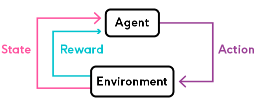
source: https://phrasee.co/
Deep Reinforcement Learning (using Deep Neural Networks for choosing actions) achieved some great things lately:
Markov Decision Processes
Markov Decision Process (MDP) is a mathematical formulation of the RL problem. MDPs satisfy the Markov property:
Markov property - the current state completely represents the state of the environment (world). That is, the future depends only on the present.
An MDP can be defined by (S,A,R,P,γ) where:
- S - set of possible states
- A - set of possible actions
- R - probability distribution of reward given (state, action) pair
- P - probability distribution over how likely any of the states is to be the new states, given (state, action) pair. Also known as transition probability.
- γ - reward discount factor
The discount factor γ allows us to inject the heuristic that 100 bucks now are more valuable than 100 bucks in 30 days. A discount factor of 1 would make future rewards worth just as much as immediate rewards.
Another reason to discount future rewards:
In the long run we are all dead - J. M. Keynes
Learning
Here is how learning happens in RL context:
for time step t=0 until done:
- The environment gives your agent a state
- Your agent chooses an action (from a set of possible ones)
- The environment gives a reward along with a new state
- Continue until the goal or other condition is met
What is the objective of all this? Find a function π∗, known as optimal policy, that maximizes the cumulative discounted reward:
t≥0∑γtrtwhere rt is the reward received at step t and γt is the discount factor at step t.
A policy π is a function that maps state s to action a, that our agent believes is the best given that state.
Value function
The value function gives you the maximum expected future reward the agent will get, starting from some state s and following some policy π.
Vπ(s)=Eπ[k=0∑∞γkRt+k+1∣St=s]There exists an optimal value function that has the highest value for all states. Defined as:
V∗(s)=πmaxVπ(s)∀s∈SQ-function
Similarly, let’s define another function known as Q-function (state-action value function) that gives the expected return starting from state s, taking action a, and following policy π.
Qπ(s,a)=Eπ[k=0∑∞γkRt+k+1∣St=s,At=a]You can think of the Q-function as the “quality” of a certain action given a state. We can define the optimal Q-function as:
Q∗(s,a)=πmaxQπ(s,a)∀s∈SThere is a relationship between the two optimal functions V∗ and Q∗. It is given by:
V∗(s)=amaxQ∗(s,a)∀s∈SThat is, the maximum expected total reward when starting at s is the maximum of Q∗(s,a) over all possible actions.
We can find the optimal policy π∗ by choosing the action a that gives maximum reward Q∗(s,a) for state s:
π∗(s)=argamaxQ∗(s,a)∀s∈SThere seems to be a synergy between all functions we defined so far. More importantly, we can now build an optimal agent for a given environment. Can we do it in practice?
Q-learning
Q-Learning is an off-policy algorithm for Temporal Difference (TD) learning. It is proven that with enough training, it converges with probability 1 to a close approximation of the action-value function for an arbitrary target policy. It learns the optimal policy even when actions are selected using exploratory (some randomness) policy (off-policy).
Given a state s and action a, we can express Q(s,a) in terms of itself (recursively):
Q(s,a)=r+γa′maxQ(s′,a′)This is the Bellman equation. It defines the maximum future reward as the reward r the agent received, for being at state s, plus the maximum future reward for state s′ for every possible action.
We can define Q-learning as an iterative approximation of Q∗ using the Bellman equation:
Qt+1(st,at)=Qt(st,at)+α(rt+1+γamaxQt(st+1,a)−Qt(st,at))where α is the learning rate that controls how much the difference between previous and new Q value is considered.
Here’s the general algorithm we’re going to implement:
- Initialize a Q-values table
- Observe initial state s
- Choose action a and act
- Observe reward r and a new state s′
- Update the Q table using r and the maximum possible reward from s′
- Set the current state to the new state and repeat from step 2 until a terminal state
Note that Q-learning is just one possible algorithm to solve the RL problem. Here is a comparison between some more of them.
Exploration vs exploitation
You might’ve noticed that we glanced over the strategy on choosing an action. Any strategy you implement will have to choose how often to try something new or use something it already knows. This is known as the exploration/exploitation tradeoff.
- Exploration - finding new information about the environment
- Exploitation - using existing information to maximize the reward
Remember, the goal of our RL agent is to maximize the expected cumulative reward. What does this mean for our self-driving taxi?
Initially, our driving agent knows pretty much nothing about the best set of driving directions for picking up and dropping off passengers. It should learn to avoid anomalies too since they are bad for business (passengers tend to disappear or worse in those)! During this time, we expect to make a lot of exploration.
After obtaining some experience, the agent can use it to choose an action more and more often. Eventually, all choices will be based on what is learned.
Driving in a post-apocalyptic world
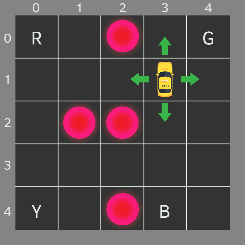
Your partner sketched this map. Each block represents a small region of the city. Anomalies are marked in bright circles. The four letters are “safe zones”, where pickups and drop-offs happen.
Let’s assume your car is the only vehicle in the city (not much of a stretch). We can break it up into a 5x5 grid, which gives us 25 possible taxi locations.
The current taxi location is (3, 1) in (row, col) coordinates. The pickup and drop off locations are: [(0,0), (0,4), (4,0), (4,3)]. Anomalies are at [(0, 2), (2, 1), (2, 2), (4, 2)].
Environment
We’re going to encode our city map into an environment for the self-driving agent using OpenAI’s Gym. What is this Gym thing anyways?
Gym is a toolkit for developing and comparing reinforcement learning algorithms. It supports teaching agents everything from walking to playing games like Pong or Pinball.
The most important entity in Gym is the Environment. It provides a unified and easy to use interface. Here are the most important methods:
reset- resets the environment and returns a random initial statestep(action)- take action and advance one timestep. It returns:observation - the new state of the environment
reward - reward received from taking the action
done - most environments are divided into well-defined episodes and if
doneisTrueit indicates the episode has been completedinfo - additional information about the environment (might be useful for debugging)
render- renders one frame of the environment (useful for visualization)
The complete source code of the environment is in the notebook. Here, we’ll take a look at the registration to Gym:
1register(2 id='SafeCab-v0',3 entry_point=f"{__name__}:SafeCab",4 timestep_limit=100,5)Note that we set a timestep_limit which limits the number of steps in an episode.
Action Space
Our agent encounters one of the 500 states (5 rows x 5 columns x 5 passanger locations x 4 destinations) and it chooses an action. Here are the possible actions:
- south
- north
- east
- west
- pickup
- dropoff
You might notice that in the illustration above, the taxi cannot perform certain actions when near the boundaries of the city. We will penalize this with -1 and won’t move the taxi if such situation occurs.
Getting a taste of the environment
Let’s have a look at our encoded environment:
1env.reset()2env.render()34print("Action Space {}".format(env.action_space))5print("State Space {}".format(env.observation_space))
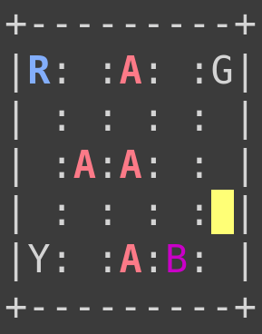
1Action Space Discrete(6)2State Space Discrete(500)Here is the action to number mapping:
- 0 = south
- 1 = north
- 2 = east
- 3 = west
- 4 = pickup
- 5 = dropoff
Building an agent
Our agent has a simple interface for interacting with the environment. Here it is:
1class Agent:23 def __init__(4 self,5 n_states,6 n_actions,7 decay_rate=0.0001,8 learning_rate=0.7,9 gamma=0.61810 ):11 pass1213 def choose_action(self, explore=True):14 pass1516 def learn(17 self,18 state,19 action,20 reward,21 next_state,22 done,23 episode24 ):25 passWe’re going to use the choose_action method when we want our agent to make a decision and act. Then, after the reward and new state from the environment are observed, our agent will learn from its actions using the learn method.
Let’s take a look at the implementations:
1def __init__(2 self,3 n_states,4 n_actions,5 decay_rate=0.0001,6 learning_rate=0.7,7 gamma=0.6188):9 self.n_actions = n_actions10 self.q_table = np.zeros((n_states, n_actions))11 self.max_epsilon = 1.012 self.min_epsilon = 0.0113 self.epsilon = self.max_epsilon14 self.decay_rate = decay_rate15 self.learning_rate = learning_rate16 self.gamma = gamma # discount rate17 self.epsilons_ = []The interesting part of the __init__ is the initialization of our Q-table. Initially, it is all zeros. Can we initialize it in some other way?
1def choose_action(self, explore=True):2 exploration_tradeoff = np.random.uniform(0, 1)34 if explore and exploration_tradeoff < self.epsilon:5 # exploration6 return np.random.randint(self.n_actions)7 else:8 # exploitation (taking the biggest Q value for this state)9 return np.argmax(self.q_table[state, :])Our strategy is rather simple. We draw a random number from a uniform distribution between 0 and 1. If this number is smaller than epsilon and we want to explore, we take a random action. Otherwise, we take the best action based on our current knowledge.
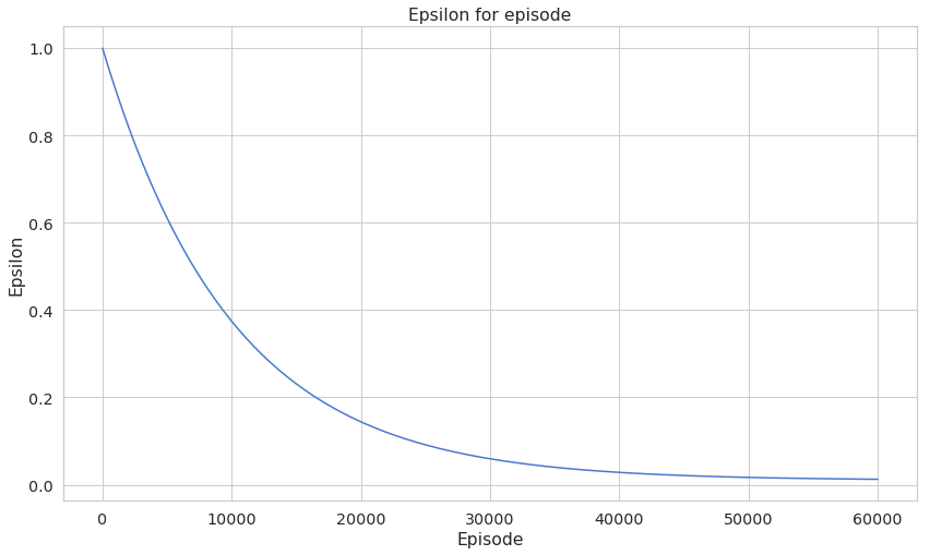
1def learn(2 self,3 state,4 action,5 reward,6 next_state,7 done,8 episode9):10 # Update Q(s,a):= Q(s,a) + lr [R(s,a) + gamma * max Q(s',a') - Q(s,a)]11 self.q_table[state, action] = self.q_table[state, action] + \12 self.learning_rate * (reward + self.gamma * \13 np.max(self.q_table[new_state, :]) - self.q_table[state, action])1415 if done:16 # Reduce epsilon to decrease the exploration over time17 self.epsilon = self.min_epsilon + (self.max_epsilon - self.min_epsilon) * \18 np.exp(-self.decay_rate * episode)19 self.epsilons_.append(self.epsilon)Learning involves the update of the Q-table using the Q-learning equation and reducing the exploration rate ϵ if the episode is complete.
Training
Now that our agent is ready for action, we can train it on the environment we’ve created. Let’s train our agent for 50k episodes and record episode rewards over time:
1total_episodes = 600002total_test_episodes = 1034agent = Agent(env.observation_space.n, env.action_space.n)Let’s have a look at our agent driving before learning anything about the environment:
1rewards = []23for episode in range(total_episodes):4 state = env.reset()5 episode_rewards = []67 while True:89 action = agent.choose_action()1011 # Take the action (a) and observe the outcome state(s') and reward (r)12 new_state, reward, done, info = env.step(action)1314 agent.learn(15 state,16 action,17 reward,18 new_state,19 done,20 episode21 )2223 state = new_state2425 episode_rewards.append(reward)2627 if done == True:28 break2930 rewards.append(np.mean(episode_rewards))Recall that we set timestep_limit when we registered the environment so our agent won’t stay in an episode infinitely.
Evaluation
Let’s have a look at reward changes as the training progresses:
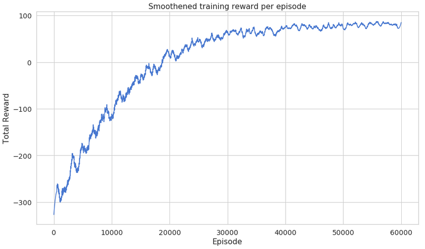
Note that the learning curve is smoothened using savgol_filter savgol_filter(rewards, window_length=1001, polyorder=2)
Recall that our exploration rate should decrease as our agent is learning. Have a look:
Here’s how we’re going to test our agent and record the progress:
1frames = []23rewards = []45for episode in range(total_test_episodes):6 state = env.reset()7 episode_rewards = []89 step = 11011 while True:12 action = agent.choose_action(explore=False)1314 new_state, reward, done, info = env.step(action)1516 frames.append({17 'frame': env.render(mode='ansi'),18 'state': state,19 'episode': episode + 1,20 'step': step,21 'reward': reward22 })2324 episode_rewards.append(reward)2526 if done:27 step = 028 break29 state = new_state30 step += 13132 rewards.append(np.mean(episode_rewards))3334env.close()Note that we want our agent to use only the experience it has so we set explore=False. Here’s what the total reward for each episode looks like:
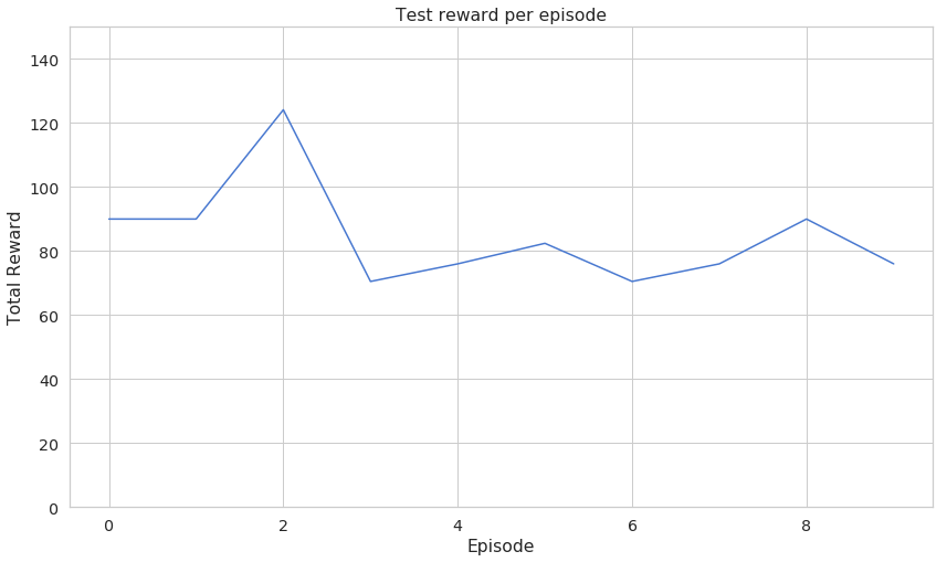
I know that this chart might not give you a good idea of what the agent is capable of. Here is a video of it driving in the city:
Pretty good, right? It looks like that it learned to avoid the anomalies, pick up and drop off passengers.
Conclusion
Congratulations on building a a self-driving taxi agent. You’ve learned how to
- Build your own environment based on one provided by OpenAI’s Gym
- Implement and apply Q-learning
- Build an agent that learns to pickup, drop off passengers and avoid danger areas
Complete source code in Google Colaboratory Notebook
Can you increase the size of the city? Does the agent learns well still? Tell me how it went in the comments below!
Share
Want to be a Machine Learning expert?
You'll never get spam from me