TL;DR Step-by-step guide to build a Deep Neural Network model with Keras to predict Airbnb prices in NYC and deploy it as REST API using Flask

This guide will let you deploy a Machine Learning model starting from zero. Here are the steps you’re going to cover:

• Define your goal
• Load data
• Data exploration
• Data preparation
• Build and evalute your model
• Save the model
• Build REST API
• Deploy to production

There is a lot to cover, but every step of the way will get you closer to deploying your model to the real-world. Let’s begin!

Run the modeling code in your browser

The complete project on GitHub

Define objective/goal

Obviously, you need to know why you need a Machine Learning (ML) model in the first place. Knowing the objective gives you insights about:

• Is ML the right approach?
• What data do I need?
• What a “good model” will look like? What metrics can I use?
• How do I solve the problem right now? How accurate is the solution?
• How much is it going to cost to keep this model running?

In our example, we’re trying to predict Airbnb listing price per night in NYC. Our objective is clear - given some data, we want our model to predict how much will it cost to rent a certain property per night.

Load data

The data comes from Airbnb Open Data and it is hosted on Kaggle

Since 2008, guests and hosts have used Airbnb to expand on traveling possibilities and present more unique, personalized way of experiencing the world. This dataset describes the listing activity and metrics in NYC, NY for 2019.

Setup

We’ll start with a bunch of imports and setting a random seed for reproducibility:

1import numpy as np
2import tensorflow as tf
3from tensorflow import keras
4import pandas as pd
5import seaborn as sns
6from pylab import rcParams
7import matplotlib.pyplot as plt
8from matplotlib import rc
9from sklearn.model_selection import train_test_split
10import joblib
11
12%matplotlib inline
13%config InlineBackend.figure_format='retina'
14
15sns.set(style='whitegrid', palette='muted', font_scale=1.5)
16
17rcParams['figure.figsize'] = 16, 10
18
19RANDOM_SEED = 42
20
21np.random.seed(RANDOM_SEED)
22tf.random.set_seed(RANDOM_SEED)

Download the data from Google Drive with gdown:

1!gdown --id 1aRXGcJlIkuC6uj1iLqzi9DQQS-3GPwM_ --output airbnb_nyc.csv

And load it into a Pandas DataFrame:

1df = pd.read_csv('airbnb_nyc.csv')

How can we understand what our data is all about?

Data exploration

This step is crucial. The goal is to get a better understanding of the data. You might be tempted to jumpstart the modeling process, but that would be suboptimal. Looking at large amounts of examples, looking for patterns and visualizing distributions will build your intuition about the data. That intuition will be helpful when modeling, imputing missing data and looking at outliers.

One easy way to start is to count the number of rows and columns in your dataset:

1df.shape

1(48895, 16)

We have 48,895 rows and 16 columns. Enough data to do something interesting.

Let’s start with the variable we’re trying to predict price. To plot the distribution, we’ll use distplot():

1sns.distplot(df.price)

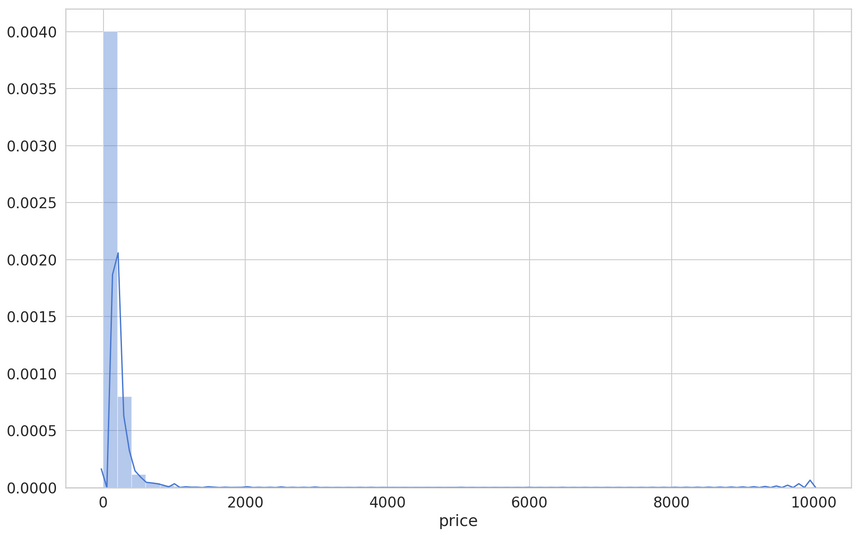
We have a highly skewed distribution with some values in the 10,000 range (you might want to explore those). We’ll use a trick - log transformation:

1sns.distplot(np.log1p(df.price))

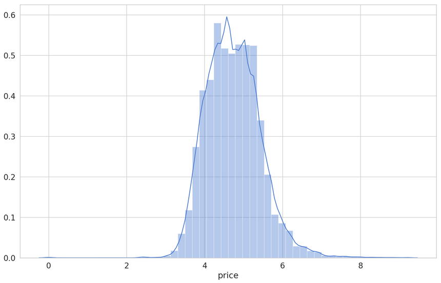
This looks more like a normal distribution. Turns out this might help your model better learn the data. You’ll have to remember to preprocess the data before training and predicting.

The type of room seems like another interesting point. Let’s have a look:

1sns.countplot(x='room_type', data=df)

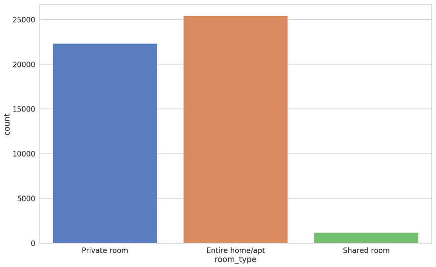
Most listings are offering entire places or private rooms. What about the location? What neighborhood groups are most represented?

1sns.countplot(x='neighbourhood_group', data=df)

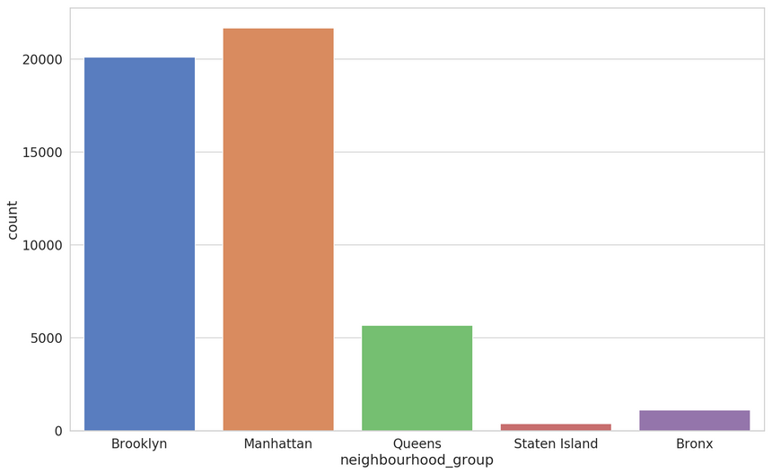
As expected, Manhattan leads the way. Obviously, Brooklyn is very well represented, too. You can thank Mos Def, Nas, Masta Ace, and Fabolous for that.

Another interesting feature is the number of reviews. Let’s have a look at it:

1sns.distplot(df.number_of_reviews)

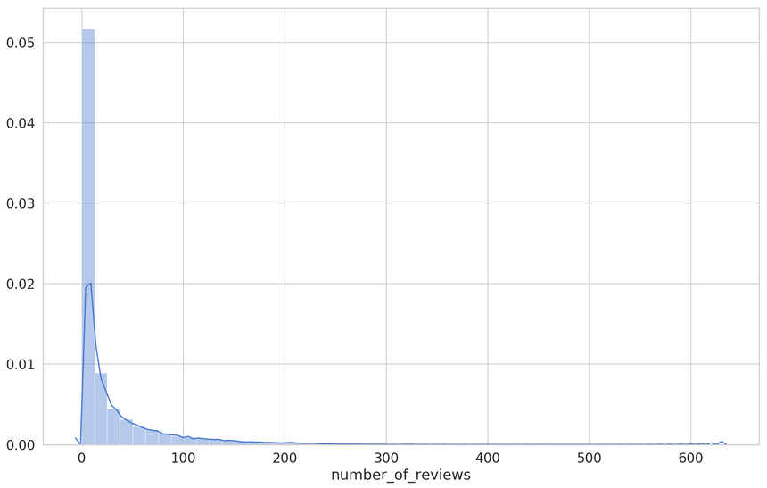
This one seems to follow a Power law (it has a fat tail). This one seems to follow a Power law (it has a fat tail). There seem to be some outliers (on the right) that might be of interest for investigation.

Finding Correlations

The correlation analysis might give you hints at what features might have predictive power when training your model.

Remember, Correlation does not imply causation

Computing Pearson correlation coefficient between a pair of features is easy:

1corr_matrix = df.corr()

Let’s look at the correlation of the price with the other attributes:

1price_corr = corr_matrix['price']
2price_corr.iloc[price_corr.abs().argsort()]

1latitude                          0.033939
2minimum_nights                    0.042799
3number_of_reviews                -0.047954
4calculated_host_listings_count    0.057472
5availability_365                  0.081829
6longitude                        -0.150019
7price                             1.000000

The correlation coefficient is defined in the -1 to 1 range. A value close to 0 means there is no correlation. Value of 1 suggests a perfect positive correlation (e.g. as the price of Bitcoin increases, your dreams of owning more are going up, too!). Value of -1 suggests perfect negative correlation (e.g. high number of bad reviews should correlate with lower prices).

The correlation in our dataset looks really bad. Luckily, categorical features are not included here. They might have some predictive power too! How can we use them?

Prepare the data

The goal here is to transform the data into a form that is suitable for your model. There are several things you want to do when handling (think CSV, Database) structured data:

• Handle missing data
• Remove unnecessary columns
• Transform any categorical features to numbers/vectors
• Scale numerical features

Missing data

Let’s start with a check for missing data:

1missing = df.isnull().sum()
2missing[missing > 0].sort_values(ascending=False)

1reviews_per_month    10052
2last_review          10052
3host_name               21
4name                    16

We’ll just go ahead and remove those features for this example. In real-world applications, you should consider other approaches.

1df = df.drop([
2    'id', 'name', 'host_id', 'host_name',
3    'reviews_per_month', 'last_review', 'neighbourhood'
4], axis=1)

We’re also dropping the neighbourhood, host id (too many unique values), and the id of the listing.

Next, we’re splitting the data into features we’re going to use for the prediction and a target variable y (the price):

1X = df.drop('price', axis=1)
2y = np.log1p(df.price.values)

Note that we’re applying the log transformation to the price.

Feature scaling and categorical data

Let’s start with feature scaling. Specifically, we’ll do min-max normalization and scale the features in the 0-1 range. Luckily, the MinMaxScaler from scikit-learn does just that.

But why do feature scaling at all? Largely because of the algorithm we’re going to use to train our model will do better with it.

Next, we need to preprocess the categorical data. Why?

Some Machine Learning algorithms can operate on categorical data without any preprocessing (like Decision trees, Naive Bayes). But most can’t.

Unfortunately, you can’t replace the category names with a number. Converting Brooklyn to 1 and Manhattan to 2 suggests that Manhattan is greater (2 times) than Brooklyn. That doesn’t make sense. How can we solve this?

We can use One-hot encoding. To get a feel of what it does, we’ll use OneHotEncoder from scikit-learn:

1from sklearn.preprocessing import OneHotEncoder
2
3data = [['Manhattan'], ['Brooklyn']]
4
5OneHotEncoder(sparse=False).fit_transform(data)

1array([[0., 1.],
2       [1., 0.]])

Essentially, you get a vector for each value that contains 1 at the index of the category and 0 for every other value. This encoding solves the comparison issue. The negative part is that your data now might take much more memory.

All data preprocessing steps are to be performed on the training data and data we’re going to receive via the REST API for prediction. We can unite the steps using make_column_transformer():

1from sklearn.preprocessing import MinMaxScaler, OneHotEncoder
2from sklearn.compose import make_column_transformer
3
4transformer = make_column_transformer(
5    (MinMaxScaler(), [
6      'latitude', 'longitude', 'minimum_nights',
7      'number_of_reviews', 'calculated_host_listings_count', 'availability_365'
8    ]),
9    (OneHotEncoder(handle_unknown="ignore"), [
10      'neighbourhood_group', 'room_type'
11    ])
12)

We enumerate all columns that need feature scaling and one-hot encoding. Those columns will be replaced with the ones from the preprocessing steps. Next, we’ll learn the ranges and categorical mapping using our transformer:

1transformer.fit(X)

Finally, we’ll transform our data:

1transformer.transform(X)

The last thing is to separate the data into training and test sets:

1X_train, X_test, y_train, y_test =\
2 train_test_split(X, y, test_size=0.2, random_state=RANDOM_SEED)

You’re going to use only the training set while developing and evaluating your model. The test set will be used later.

That’s it! You are now ready to build a model. How can you do that?

Build your model

Finally, it is time to do some modeling. Recall the goal we set for ourselves at the beginning:

We’re trying to predict Airbnb listing price per night in NYC

We have a price prediction problem on our hands. More generally, we’re trying to predict a numerical value defined in a very large range. This fits nicely in the Regression Analysis framework.

Training a model boils down to minimizing some predefined error. What error should we measure?

Error measurement

We’ll use Mean Squared Error which measures the difference between average squared predicted and true values:

where $n$ is the number of samples, $Y$ is a vector containing the real values and $\hat{Y}$ is a vector containing the predictions from our model.

Now that you have a measurement of how well your model is performing is time to build the model itself. How can you build a Deep Neural Network with Keras?

Build a Deep Neural Network with Keras

Keras is the official high-level API for TensorFlow. In short, it allows you to build complex models using a sweet interface. Let’s build a model with it:

1model = keras.Sequential()
2model.add(keras.layers.Dense(
3  units=64,
4  activation="relu",
5  input_shape=[X_train.shape[1]]
6))
7model.add(keras.layers.Dropout(rate=0.3))
8model.add(keras.layers.Dense(units=32, activation="relu"))
9model.add(keras.layers.Dropout(rate=0.5))
10
11model.add(keras.layers.Dense(1))

The sequential API allows you to add various layers to your model, easily. Note that we specify the input_size in the first layer using the training data. We also do regularization using Dropout layers.

How can we specify the error metric?

1model.compile(
2    optimizer=keras.optimizers.Adam(0.0001),
3    loss = 'mae',
4    metrics = ['mae'])

The compile() method lets you specify the optimizer and the error metric you need to reduce.

Your model is ready for training. Let’s go!

Training

Training a Keras model involves calling a single method - fit():

1BATCH_SIZE = 32
2
3early_stop = keras.callbacks.EarlyStopping(
4  monitor='val_mae',
5  mode="min",
6  patience=10
7)
8
9history = model.fit(
10  x=X_train,
11  y=y_train,
12  shuffle=True,
13  epochs=100,
14  validation_split=0.2,
15  batch_size=BATCH_SIZE,
16  callbacks=[early_stop]
17)

We feed the training method with the training data and specify the following parameters:

• shuffle - random sort the data
• epochs - number of training cycles
• validation_split - use some percent of the data for measuring the error and not during training
• batch_size - the number of training examples that are fed at a time to our model
• callbacks - we use EarlyStopping to prevent our model from overfitting when the training and validation error start to diverge

After the long training process is complete, you need to answer one question. Can your model make good predictions?

Evaluation

One simple way to understand the training process is to look at the training and validation loss:

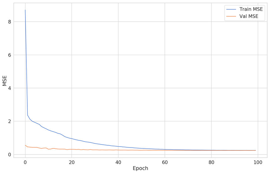
We can see a large improvement in the training error, but not much on the validation error. What else can we use to test our model?

Using the test data

Recall that we have some additional data. Now it is time to use it and test how good our model. Note that we don’t use that data during the training, only once at the end of the process.

Let’s get the predictions from the model:

1y_pred = model.predict(X_test)

And we’ll use a couple of metrics for the evaluation:

1from sklearn.metrics import mean_squared_error
2from math import sqrt
3from sklearn.metrics import r2_score
4
5print(f'MSE {mean_squared_error(y_test, y_pred)}')
6print(f'RMSE {np.sqrt(mean_squared_error(y_test, y_pred))}')

1MSE 0.2139184014903989
2RMSE 0.4625131365598159

We’ve already discussed MSE. You can probably guess what Root Mean Squared Error (RMSE) means. RMSE allows us to penalize points further from the mean.

Another statistic we can use to measure how well our predictions fit with the real data is the $R^2$ score. A value close to 1 indicates a perfect fit. Let’s check ours:

1print(f'R2 {r2_score(y_test, y_pred)}')

1R2 0.5478250409482018

There is definitely room for improvement here. You might try to tune the model better and get better results.

Now you have a model and a rough idea of how well will it do in production. How can you save your work?

Save the model

Now that you have a trained model, you need to store it and be able to reuse it later. Recall that we have a data transformer that needs to be stored, too! Let’s save both:

1import joblib
2
3joblib.dump(transformer, "data_transformer.joblib")
4model.save("price_prediction_model.h5")

The recommended approach of storing scikit-learn models is to use joblib. Saving the model architecture and weights of a Keras model is done with the save() method.

You can download the files from the notebook using the following:

1from google.colab import files
2
3files.download("data_transformer.joblib")
4files.download("price_prediction_model.h5")

Build REST API

Building a REST API allows you to use your model to make predictions for different clients. Almost any device can speak REST - Android, iOS, Web browsers, and many others.

Flask allows you to build a REST API in just a couple of lines. Of course, we’re talking about a quick-and-dirty prototype. Let’s have a look at the complete code:

1from math import expm1
2
3import joblib
4import pandas as pd
5from flask import Flask, jsonify, request
6from tensorflow import keras
7
8app = Flask(__name__)
9model = keras.models.load_model("assets/price_prediction_model.h5")
10transformer = joblib.load("assets/data_transformer.joblib")
11
12
13@app.route("/", methods=["POST"])
14def index():
15    data = request.json
16    df = pd.DataFrame(data, index=[0])
17    prediction = model.predict(transformer.transform(df))
18    predicted_price = expm1(prediction.flatten()[0])
19    return jsonify({"price": str(predicted_price)})

The complete project (including the data transformer and model) is on GitHub: Deploy Keras Deep Learning Model with Flask

The API has a single route (index) that accepts only POST requests. Note that we pre-load the data transformer and the model.

The request handler obtains the JSON data and converts it into a Pandas DataFrame. Next, we use the transformer to pre-process the data and get a prediction from our model. We invert the log operation we did in the pre-processing step and return the predicted price as JSON.

Your REST API is ready to go. Run the following command in the project directory:

1flask run

Open a new tab to test the API:

1curl -d '{"neighbourhood_group": "Brooklyn", "latitude": 40.64749, "longitude": -73.97237, "room_type": "Private room", "minimum_nights": 1, "number_of_reviews": 9, "calculated_host_listings_count": 6, "availability_365": 365}' -H "Content-Type: application/json" -X POST http://localhost:5000

You should see something like the following:

1{"price":"72.70381414559431"}

Great. How can you deploy your project and allow others to consume your model predictions?

Deploy to production

We’ll deploy the project to Google App Engine:

App Engine enables developers to stay more productive and agile by supporting popular development languages and a wide range of developer tools.

App Engine allows us to use Python and easily deploy a Flask app.

You need to:

• Register for Google Cloud Engine account
• Google Cloud SDK installed

Here is the complete app.yaml config:

1entrypoint: "gunicorn -b :$PORT app:app --timeout 500"
2runtime: python
3env: flex
4service: nyc-price-prediction
5runtime_config:
6  python_version: 3.7
7instance_class: B1
8manual_scaling:
9  instances: 1
10liveness_check:
11  path: "/liveness_check"

Execute the following command to deploy the project:

1gcloud app deploy

Wait for the process to complete and test the API running on production. You did it!

Conclusion

Your model should now be running, making predictions, and accessible to everyone. Of course, you have a quick-and-dirty prototype. You will need a way to protect and monitor your API. Maybe you need a better (automated) deployment strategy too!

Still, you have a model deployed in production and did all of the following:

• Define your goal
• Load data
• Data exploration
• Data preparation
• Build and evalute your model
• Save the model
• Build REST API
• Deploy to production

How do you deploy your models? Comment down below :)

Run the modeling code in your browser

The complete project on GitHub

References

• Joblib - running Python functions as pipeline jobs
• Flask - lightweight web application framework
• Building a simple Keras + deep learning REST API