Curiousily

Diagnosing Breast Cancer from Image Data

05.10.2016 — R, Classification — 2 min read

Detecting breast (or any other type of) cancer before noticing symptoms is a key first step in fighting the disease. The process involves examining breast tissue for lumps or masses. Fine needle aspirate (FNA) biopsy is performed if such irregularity is found. The extracted tissue is then examined under a microscope by a clinician.

Can a machine help the clinician do a better job? Can the doctor focus more on treating the disease rather than detecting it? Recently, Deep Learning (DL) has seen major advances in the area of computer vision. Naturally, some scientists tried to apply it to breast cancer detection - and did so with great success!

Here, we will look at a dataset created by Dr. William H. Wolberg, W. Nick Street and Olvi L. Mangasarian from the University of Wisconsin. Each row describes features of the cell nuclei present in the digitized image of the FNA along with the diagnosis (M = malignant, B = benign) and ID of a patient with a lump in her breast.

Here is a list of the measured cell nuclei features:

radius (mean of distances from center to points on the perimeter)
texture (standard deviation of gray-scale values)
perimeter
area
smoothness (local variation in radius lengths)
compactness (perimeter^2 / area - 1.0)
concavity (severity of concave portions of the contour)
concave points (number of concave portions of the contour)
symmetry
fractal dimension (“coastline approximation” - 1)

Can we predict whether the lump is benign or malignant?

Sample image from which the cell nuclei features are extracted

Fire up R and load some libraries

1library(ggplot2)
2library(Amelia)
3library(class)
4library(gmodels)
5
6set.seed(42)

Exploration

1df <- read.csv("data/breast_cancer.csv", stringsAsFactors = FALSE)

1print(paste("rows:", nrow(df), "cols:", ncol(df)))

1[1] "rows: 569 cols: 32"

Let’s remove the ID column and recode the diagnosis.

1df <- df[-1]
2df$diagnosis <- factor(df$diagnosis, levels = c("B", "M"),
3                         labels = c("Benign", "Malignant"))

Do we have missing data?

1missmap(df, main="Missing Data Map", col=c("#FF4081", "#3F51B5"),
2        legend=FALSE)

Nope. That’s good! What is the distribution for the both types of cancer?

1barplot(table(df$diagnosis), xlab = "Type of tumor", ylab="Numbers per type")

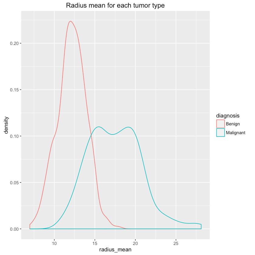
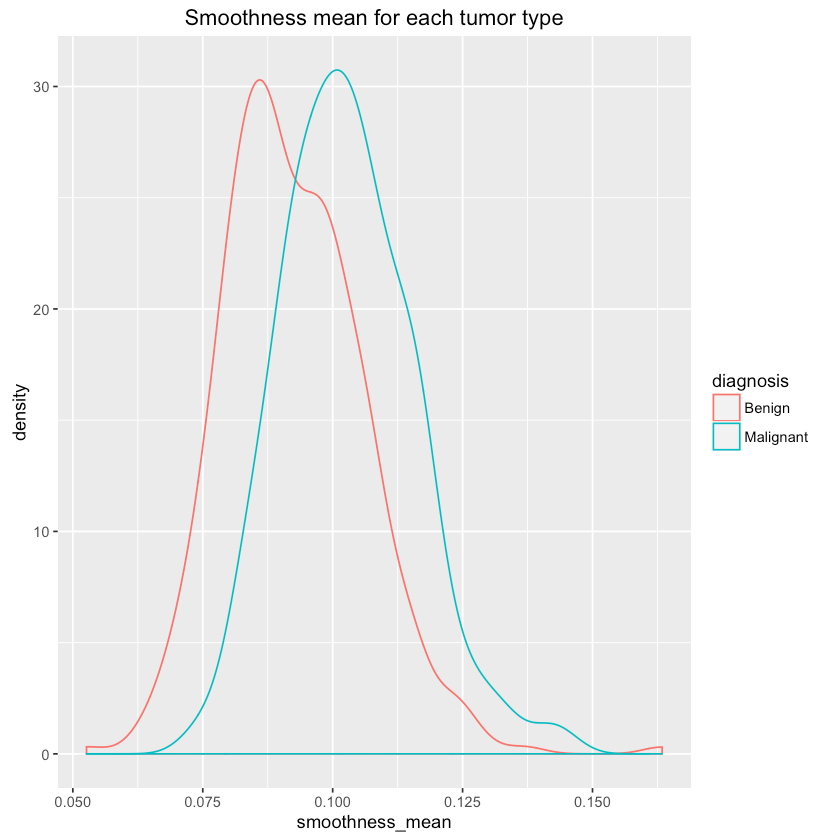
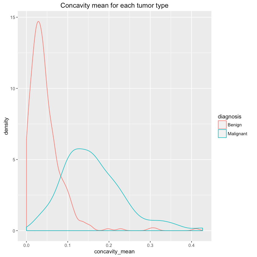
Let’s see if we can differentiate between tumor types using some features (randomly chosen?):

1qplot(radius_mean, data=df, colour=diagnosis, geom="density",
2      main="Radius mean for each tumor type")

1qplot(smoothness_mean, data=df, colour=diagnosis, geom="density",
2      main="Smoothness mean for each tumor type")

1qplot(concavity_mean, data=df, colour=diagnosis, geom="density",
2      main="Concavity mean for each tumor type")

Preprocess the data

Let’s normalize (scale every value in our dataset in the range [0:1]) our data. This will become handy when we try to classify the tumor type for each patient.

1normalize <- function(x) {
2  return ((x - min(x)) / (max(x) - min(x)))
3}
4
5df_normalized <- as.data.frame(lapply(df[2:31], normalize))

Additionaly, let’s create a scaled version of our dataset too! The formula for scaling is the following:

$\frac{x - mean(x)}{\sigma(x)}$

where $x$ is a vector that contains real numbers.

1df_scaled <- as.data.frame(scale(df[-1]))

Splitting our data

Now, let’s split our dataset into 3 new - training, test and validation. First, let’s put aside 150 rows for test/validation and use the rest for training:

1train_idx <- sample(nrow(df_normalized), nrow(df_normalized) - 150,
2                    replace = FALSE)
3df_normalized_train <- df_normalized[train_idx, ]

Let’s use 100 of the rest for testing and 50 for validation:

1test_validation_idx <- seq(1:nrow(df_normalized))[-train_idx]
2test_idx <- sample(test_validation_idx, 100, replace = FALSE)
3validation_idx <- test_validation_idx[-test_idx]
4
5df_normalized_test <- df_normalized[test_idx, ]
6df_normalized_validation <- df_normalized[validation_idx, ]

Predicting tumor type

We will use simple k-means clustering algorithm to predict whether a patient has a benign or malignant tumor.

1df_train_labels <- df[train_idx, 1]
2df_test_labels <- df[test_idx, 1]
3df_validation_labels <- df[validation_idx, 1]
4
5df_normalized_pred_labels <- knn(train = df_normalized_train,
6                                 test = df_normalized_test,
7                                 cl = df_train_labels,
8                                 k = 21)

Ok, that was quick. How did we do? Let’s evaluate our model using a cross table and see:

1evaluate_model <- function(expected_labels, predicted_labels) {
2    CrossTable(x = expected_labels, y = predicted_labels, prop.chisq=FALSE)
3    true_predctions <- table(expected_labels == predicted_labels)["TRUE"]
4    correct_predictions <- true_predictions / length(predicted_labels)
5    print(paste("Correctly predicted: ", correct_predictions))
6}

1evaluate_model(df_test_labels, df_normalized_pred_labels)

1Cell Contents
2|-------------------------|
3|                       N |
4|           N / Row Total |
5|           N / Col Total |
6|         N / Table Total |
7|-------------------------|
8
9
10Total Observations in Table:  100
11
12
13                | predicted_labels
14expected_labels |    Benign | Malignant | Row Total |
15----------------|-----------|-----------|-----------|
16         Benign |        60 |         0 |        60 |
17                |     1.000 |     0.000 |     0.600 |
18                |     0.952 |     0.000 |           |
19                |     0.600 |     0.000 |           |
20----------------|-----------|-----------|-----------|
21      Malignant |         3 |        37 |        40 |
22                |     0.075 |     0.925 |     0.400 |
23                |     0.048 |     1.000 |           |
24                |     0.030 |     0.370 |           |
25----------------|-----------|-----------|-----------|
26   Column Total |        63 |        37 |       100 |
27                |     0.630 |     0.370 |           |
28----------------|-----------|-----------|-----------|
29
30
31[1] "Correctly predicted:  0.97"

Not bad, only 3 errors. Can we do better? Let’s use our scaled dataset:

1df_scaled_train <- df_scaled[train_idx, ]
2df_scaled_test <- df_scaled[test_idx, ]
3df_scaled_validation <- df_scaled[validation_idx, ]

1df_scaled_pred_labels <- knn(train = df_scaled_train,
2                             test = df_scaled_test,
3                             cl = df_train_labels,
4                             k = 21)

1evaluate_model(df_test_labels, df_scaled_pred_labels)

1Cell Contents
2|-------------------------|
3|                       N |
4|           N / Row Total |
5|           N / Col Total |
6|         N / Table Total |
7|-------------------------|
8
9
10Total Observations in Table:  100
11
12
13                | predicted_labels
14expected_labels |    Benign | Malignant | Row Total |
15----------------|-----------|-----------|-----------|
16         Benign |        60 |         0 |        60 |
17                |     1.000 |     0.000 |     0.600 |
18                |     0.938 |     0.000 |           |
19                |     0.600 |     0.000 |           |
20----------------|-----------|-----------|-----------|
21      Malignant |         4 |        36 |        40 |
22                |     0.100 |     0.900 |     0.400 |
23                |     0.062 |     1.000 |           |
24                |     0.040 |     0.360 |           |
25----------------|-----------|-----------|-----------|
26   Column Total |        64 |        36 |       100 |
27                |     0.640 |     0.360 |           |
28----------------|-----------|-----------|-----------|
29
30
31[1] "Correctly predicted:  0.96"

Huh, even worse! Let’s try different k values:

1train_and_evaluate <- function(train, test, train_labels, test_labels, k) {
2    predicted_labels <- knn(train = train, test = test,
3                            cl = train_labels, k = k)
4    evaluate_model(test_labels, predicted_labels)
5}

1train_and_evaluate(df_normalized_train, df_normalized_test,
2                   df_train_labels, df_test_labels, 1)

1Cell Contents
2|-------------------------|
3|                       N |
4|           N / Row Total |
5|           N / Col Total |
6|         N / Table Total |
7|-------------------------|
8
9
10Total Observations in Table:  100
11
12
13                | predicted_labels
14expected_labels |    Benign | Malignant | Row Total |
15----------------|-----------|-----------|-----------|
16         Benign |        60 |         0 |        60 |
17                |     1.000 |     0.000 |     0.600 |
18                |     0.952 |     0.000 |           |
19                |     0.600 |     0.000 |           |
20----------------|-----------|-----------|-----------|
21      Malignant |         3 |        37 |        40 |
22                |     0.075 |     0.925 |     0.400 |
23                |     0.048 |     1.000 |           |
24                |     0.030 |     0.370 |           |
25----------------|-----------|-----------|-----------|
26   Column Total |        63 |        37 |       100 |
27                |     0.630 |     0.370 |           |
28----------------|-----------|-----------|-----------|
29
30
31[1] "Correctly predicted:  0.97"

1train_and_evaluate(df_normalized_train, df_normalized_test,
2                   df_train_labels, df_test_labels, 5)

1Cell Contents
2|-------------------------|
3|                       N |
4|           N / Row Total |
5|           N / Col Total |
6|         N / Table Total |
7|-------------------------|
8
9
10Total Observations in Table:  100
11
12
13                | predicted_labels
14expected_labels |    Benign | Malignant | Row Total |
15----------------|-----------|-----------|-----------|
16         Benign |        60 |         0 |        60 |
17                |     1.000 |     0.000 |     0.600 |
18                |     0.952 |     0.000 |           |
19                |     0.600 |     0.000 |           |
20----------------|-----------|-----------|-----------|
21      Malignant |         3 |        37 |        40 |
22                |     0.075 |     0.925 |     0.400 |
23                |     0.048 |     1.000 |           |
24                |     0.030 |     0.370 |           |
25----------------|-----------|-----------|-----------|
26   Column Total |        63 |        37 |       100 |
27                |     0.630 |     0.370 |           |
28----------------|-----------|-----------|-----------|
29
30
31[1] "Correctly predicted:  0.97"

1train_and_evaluate(df_normalized_train, df_normalized_test,
2                   df_train_labels, df_test_labels, 15)

1Cell Contents
2|-------------------------|
3|                       N |
4|           N / Row Total |
5|           N / Col Total |
6|         N / Table Total |
7|-------------------------|
8
9
10Total Observations in Table:  100
11
12
13                | predicted_labels
14expected_labels |    Benign | Malignant | Row Total |
15----------------|-----------|-----------|-----------|
16         Benign |        60 |         0 |        60 |
17                |     1.000 |     0.000 |     0.600 |
18                |     0.952 |     0.000 |           |
19                |     0.600 |     0.000 |           |
20----------------|-----------|-----------|-----------|
21      Malignant |         3 |        37 |        40 |
22                |     0.075 |     0.925 |     0.400 |
23                |     0.048 |     1.000 |           |
24                |     0.030 |     0.370 |           |
25----------------|-----------|-----------|-----------|
26   Column Total |        63 |        37 |       100 |
27                |     0.630 |     0.370 |           |
28----------------|-----------|-----------|-----------|
29
30
31[1] "Correctly predicted:  0.97"

Not much change. Let’s see how our model performs on the validation set:

1train_and_evaluate(df_normalized_train, df_normalized_validation,
2                   df_train_labels, df_validation_labels, 21)

1Cell Contents
2|-------------------------|
3|                       N |
4|           N / Row Total |
5|           N / Col Total |
6|         N / Table Total |
7|-------------------------|
8
9
10Total Observations in Table:  127
11
12
13                | predicted_labels
14expected_labels |    Benign | Malignant | Row Total |
15----------------|-----------|-----------|-----------|
16         Benign |        79 |         0 |        79 |
17                |     1.000 |     0.000 |     0.622 |
18                |     0.929 |     0.000 |           |
19                |     0.622 |     0.000 |           |
20----------------|-----------|-----------|-----------|
21      Malignant |         6 |        42 |        48 |
22                |     0.125 |     0.875 |     0.378 |
23                |     0.071 |     1.000 |           |
24                |     0.047 |     0.331 |           |
25----------------|-----------|-----------|-----------|
26   Column Total |        85 |        42 |       127 |
27                |     0.669 |     0.331 |           |
28----------------|-----------|-----------|-----------|
29
30
31[1] "Correctly predicted:  0.952755905511811"

Our final accuracy is about 95%. What does this mean? If our model was to replace a doctor it would missclassify 6 malignant tumors as benign. This is bad! The other type of error (missclassifying benign tumor as malignant) is pretty bad too! So, improvement to the accuracy (in any way) might save lives! Can you improve the model?

P. S. This post was written as an ipython notebook. Download it from here. The dataset can be download from here.

Want to be a Machine Learning expert?

Join the weekly newsletter on Data Science, Deep Learning and Machine Learning in your inbox, curated by me! Chosen by 10,000+ Machine Learning practitioners. (There might be some exclusive content, too!)

You'll never get spam from me

Hacker's Guide to Neural Networks in JavaScript

Build Machine Learning models (especially Deep Neural Networks) that you can easily integrate with existing or new web apps. Think of your ReactJs, Vue, or Angular app enhanced with the power of Machine Learning models.

Get SH*T Done with PyTorch

Learn how to solve real-world problems with Deep Learning models (NLP, Computer Vision, and Time Series). Go from prototyping to deployment with PyTorch and Python!

Hacker's Guide to Machine Learning with Python

This book brings the fundamentals of Machine Learning to you, using tools and techniques used to solve real-world problems in Computer Vision, Natural Language Processing, and Time Series analysis. The skills taught in this book will lay the foundation for you to advance your journey to Machine Learning Mastery!

Hands-On Machine Learning from Scratch

This book will guide you on your journey to deeper Machine Learning understanding by developing algorithms in Python from scratch! Learn why and when Machine learning is the right tool for the job and how to improve low performing models!