Fashion product image classification using Neural Networks | Machine Learning from Scratch (Part VI)
— Machine Learning, Computer Vision, Neural Networks, Image Classification — 7 min read
Share
TL;DR Build Neural Network in Python from scratch. Use the model to classify images of fashion products into 1 of 10 classes.
We live in the age of Instagram, YouTube, and Twitter. Images and video (a sequence of images) dominate the way millennials and other weirdos consume information.
Having models that understand what images show can be crucial for understanding your emotional state (yes, you might get a personalized Coke ad right after you post your breakup selfie on Instagram), location, interests and social group.
Predominantly, models that understand image data used in practice are (Deep) Neural Networks. Here, we’ll implement a Neural Network image classifier from scratch in Python.
Complete source code in Google Colaboratory Notebook
Image Data
Hopefully, it’s not a complete surprise to you that computers can’t actually see images as we do. Each image on your device is represented/stored as a matrix, where each pixel is one or more numbers.
Reading the fashion products data
Fashion-MNIST is a dataset of Zalando’s article images—consisting of a training set of 60,000 examples and a test set of 10,000 examples. Each example is a 28x28 grayscale image, associated with a label from 10 classes. We intend Fashion-MNIST to serve as a direct drop-in replacement for the original MNIST dataset for benchmarking machine learning algorithms. It shares the same image size and structure of training and testing splits.
Here is a sample of the images:
![]()
You might be familiar with the original handwritten digits MNIST dataset and wondering why we’re not using it? Well, it might be too easy to make predictions on. And of course, fashion is cooler, right?
Exploration
The product images are grayscale, 28x28 pixels and look something like this:
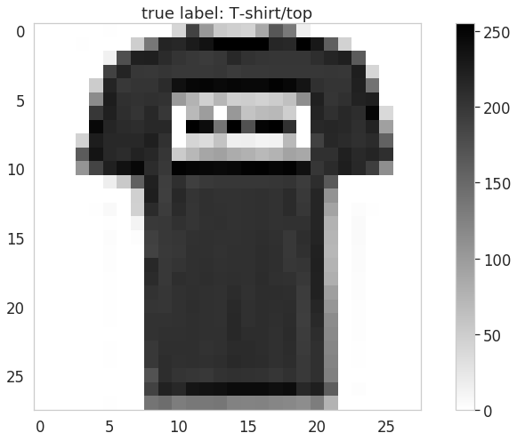
Here are the first 3 rows from the pixel matrix of the image:
1[[ 0, 0, 0, 0, 0, 1, 0, 0, 0, 0, 41, 188, 103,2 54, 48, 43, 87, 168, 133, 16, 0, 0, 0, 0, 0, 0,3 0, 0],4 [ 0, 0, 0, 1, 0, 0, 0, 49, 136, 219, 216, 228, 236,5 255, 255, 255, 255, 217, 215, 254, 231, 160, 45, 0, 0, 0,6 0, 0],7 [ 0, 0, 0, 0, 0, 14, 176, 222, 224, 212, 203, 198, 196,8 200, 215, 204, 202, 201, 201, 201, 209, 218, 224, 164, 0, 0,9 0, 0],10 ...11]Note that the values are in the 0-255 range (grayscale).
We have 10 classes of possible fashion products:
1['T-shirt/top', 'Trouser', 'Pullover', 'Dress', 'Coat',2 'Sandal', 'Shirt', 'Sneaker', 'Bag', 'Ankle boot']Let’s have a look at a lower dimensional representation of some of the products using t-SNE. We’ll transform the data into 2-dimensional using the implementation from scikit-learn:
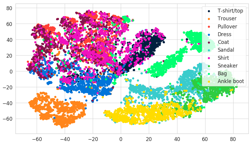
You can observe a clear separation between some classes and significant overlap between others. Let’s build a Neural Network that can try to separate between different fashion products!
Neural Networks
Neural Networks (NNs), Deep Neural Networks in particular, are all the rage in the last couple of years in the Machine Learning realm. That’s hardly a surprise since most state-of-the-art results (SOTA) on various Machine Learning problems are obtained via Neural Nets.
The Artificial Neuron
The goal of modeling our biological neuron has led to the invention of the artificial neuron. Here is how a single neuron in your brain looks like:
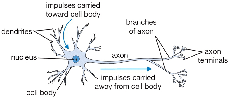
source: CS231n
On the other side, we have a vastly simplified mathematical model that turns out to be extremely useful in practice (as evident by the success of Neural Nets):
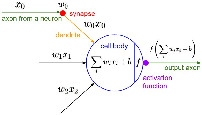
source: CS231n
The idea of the artificial neuron is simple - you have data vector X coming from somewhere, a vector of parameters W and a bias vector b. The output of a neuron is given by:
Y=f(i∑wixi+b)where f is an activation function that controls how strong the output signal of the neuron is.
Architecting Neural Networks
You can use a single neuron as a classifier, but the fun part begins when you group them into layers. Concretely, the neurons are connected into an acyclic graph with the data flowing between layers:
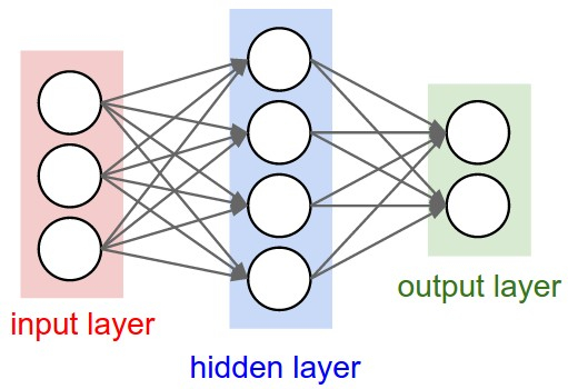
source: CS231n
This simple Neural Network contains:
- Input layer - 3 neurons that should match the size of your input data
- Hidden layer - 4 neurons with weights W that your model should learn during training
- Output layer - 2 neurons that provide the predictions of your model
Want to build a Deep Neural Network? Just add at least one more hidden layer:
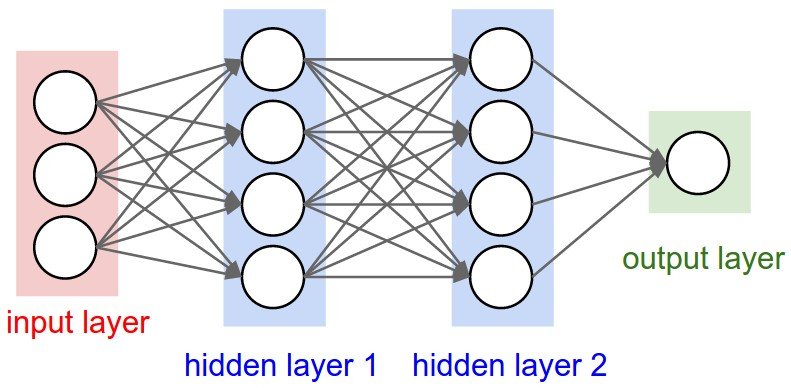
source: CS231n
Sigmoid
The sigmoid function is quite commonly used activation function, at least it was until recently. It has a distinct S shape, it is a differentiable real function for any real input value and output values between 0 and 1. Additionally, it has a positive derivative at each point. More importantly, we will use it as an activation function for the hidden layer of our model.
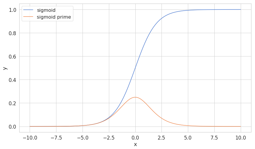
Here’s how it is defined:
σ(x)=1+e−x1Here is how we can implement it:
1def sigmoid(z):2 return 1.0 / (1.0 + np.exp(-z))Its first derivative (which we will use during the backpropagation step of our training algorithm) has the following formula:
d(x)dσ(x)=σ(x)⋅(1−σ(x))Our implementation reuses the sigmoid implementation itself:
1def sigmoid_prime(z):2 sg = sigmoid(z)3 return sg * (1 - sg)Softmax
The softmax function can be easily differentiated, it is pure (output depends only on input) and the elements of the resulting vector sum to 1. Here it is:
σ(z)j=∑Kk=1ezkezjforj=1,...,kHere is the Python implementation:
1def softmax(z):2 return (np.exp(z.T) / np.sum(np.exp(z), axis=1)).TIn probability theory, the output of the softmax function is sometimes used as a representation of a categorical distribution. Let’s see an example result:
1softmax(np.array([[2, 4, 6, 8]]))1array([[ 0.00214401, 0.0158422 , 0.11705891, 0.86495488]])The output has most of its weight corresponding to the input 8. The softmax function highlights the largest value(s) and suppresses the smaller ones.
Backpropagation
Backpropagation is the backbone of almost anything we do when using Neural Networks. The algorithm consists of 3 subtasks:
- Make a forward pass
- Calculate the error
- Make backward pass (backpropagation)
In the first step, backprop uses the data and the weights of the network to compute a prediction. Next, the error is computed based on the prediction and the provided labels. The final step propagates the error through the network, starting from the final layer. Thus, the weights get updated based on the error, little by little.
Let’s build more intuition about what the algorithm is actually doing:
Solving XOR
We will try to create a Neural Network that can properly predict values from the XOR function. Here is its truth table:
| Input 1 | Input 2 | Output |
|---|---|---|
| 0 | 0 | 0 |
| 0 | 1 | 1 |
| 1 | 0 | 1 |
| 1 | 1 | 0 |
Here is a visual representation:
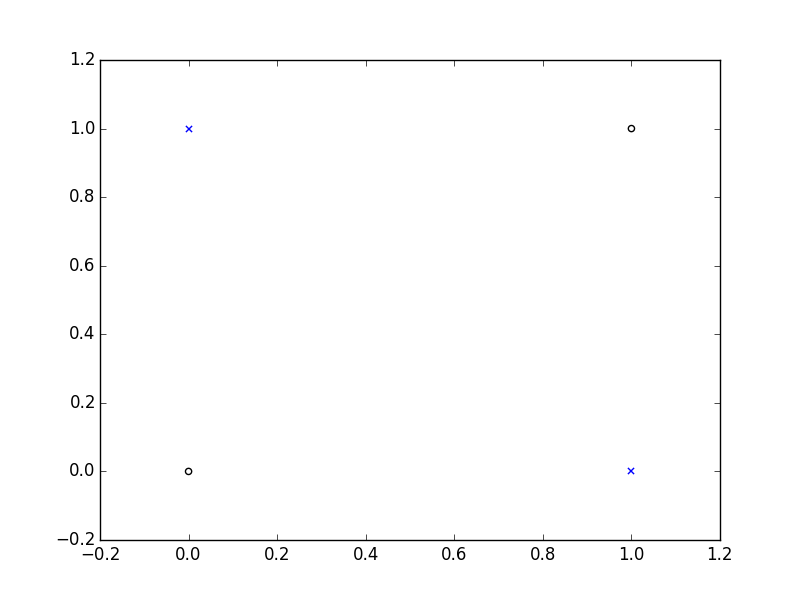
Let start by defining some parameters:
1epochs = 500002input_size, hidden_size, output_size = 2, 3, 13LR = .1 # learning rateThe epochs parameter controls how many times our algorithm will “see” the data during training. Then we set the number of neurons in the input, hidden and output layers - we have 2 numbers as input and 1 number as output size. The learning rate parameter controls how quickly our Neural Network will learn from new data and forget what already knows.
Our training data (from the table) looks like this:
1X = np.array([[0,0], [0,1], [1,0], [1,1]])2y = np.array([ [0], [1], [1], [0]])The W vectors in our NN need to have some initial values. We’ll sample a uniform distribution, initialized with proper size:
1w_hidden = np.random.uniform(size=(input_size, hidden_size))2w_output = np.random.uniform(size=(hidden_size, output_size))Finally, implementation of the Backprop algorithm:
1for epoch in range(epochs):23 # Forward4 act_hidden = sigmoid(np.dot(X, w_hidden))5 output = np.dot(act_hidden, w_output)67 # Calculate error8 error = y - output910 if epoch % 5000 == 0:11 print(f'error sum {sum(error)}')1213 # Backward14 dZ = error * LR15 w_output += act_hidden.T.dot(dZ)16 dH = dZ.dot(w_output.T) * sigmoid_prime(act_hidden)17 w_hidden += X.T.dot(dH)1error sum [-1.77496016]2error sum [ 0.00586565]3error sum [ 0.00525699]4error sum [ 0.0003625]5error sum [-0.00064657]6error sum [ 0.00189532]7error sum [ 3.79101898e-08]8error sum [ 7.47615376e-13]9error sum [ 1.40960742e-14]10error sum [ 1.49842526e-14]That error seems to be decreasing! YaY! And the implementation is not that scary, isn’t it?
During the forward step, we take the dot product of the data X and Whidden and apply our activation function to obtain the output of our hidden layer. We obtain the predictions by taking the dot product of the hidden layer output and Woutput.
To obtain the error, we calculate the difference between the true values and the predicted ones. Note that this is a very crude metric, but it works fine for our example.
Finally, we use the calculated error to adjust the weights. Note that we need the results from the forward pass act_hidden to calculate Woutput and calculate the first derivative using sigmoid_prime to update Whidden.
In order to make an inference (predictions) we’ll do just the forward step (since we won’t adjust W based on the result):
1test_data = X[1] # [0, 1]23act_hidden = sigmoid(np.dot(test_data, w_hidden))4np.dot(act_hidden, w_output)1array([ 1.])Our sorcery seems to be working! The prediction is correct!
Classifying Images
Building a Neural Network
Our Neural Network will have only 1 hidden layer. We will implement a somewhat more sophisticated version of our training algorithm shown above along with some handy methods.
Initializing the weights
We’ll sample a uniform distribution with values between -1 and 1 for our initial weights. Here is the implementation:
1def _init_weights(self):2 w1 = np.random.uniform(-1.0, 1.0,3 size=(self.n_hidden_units, self.n_features))4 w2 = np.random.uniform(-1.0, 1.0,5 size=(self.n_classes, self.n_hidden_units))6 return w1, w2Training
Let’s have a look at the training method:
1def fit(self, X, y):2 self.error_ = []3 X_data, y_data = X.copy(), y.copy()4 y_data_enc = one_hot(y_data, self.n_classes)56 X_mbs = np.array_split(X_data, self.n_batches)7 y_mbs = np.array_split(y_data_enc, self.n_batches)89 for i in range(self.epochs):1011 epoch_errors = []1213 for Xi, yi in zip(X_mbs, y_mbs):1415 # update weights16 error, grad1, grad2 = self._backprop_step(Xi, yi)17 epoch_errors.append(error)18 self.w1 -= self.learning_rate * grad119 self.w2 -= self.learning_rate * grad220 self.error_.append(np.mean(epoch_errors))21 return selfFor each epoch, we apply the backprop algorithm, evaluate the error and the gradient with respect to the weights. We then use the learning rate and gradients to update the weights.
1def _backprop_step(self, X, y):2 net_input, net_hidden, act_hidden, net_out, act_out = self._forward(X)3 y = y.T45 grad1, grad2 = self._backward(net_input, net_hidden, act_hidden, act_out, y)67 # regularize8 grad1 += self.w1 * (self.l1 + self.l2)9 grad2 += self.w2 * (self.l1 + self.l2)1011 error = self._error(y, act_out)1213 return error, grad1, grad2Doing a backprop step is a bit more complicated than our XOR example. We do an additional step before returning the gradients - apply L1 and L2 Regularization. Regularization is used to guide our training towards simpler methods by penalizing large values for our parameters W.
1def _forward(self, X):2 net_input = X.copy()3 net_hidden = self.w1.dot(net_input.T)4 act_hidden = sigmoid(net_hidden)5 net_out = self.w2.dot(act_hidden)6 act_out = sigmoid(net_out)7 return net_input, net_hidden, act_hidden, net_out, act_out89def _backward(self, net_input, net_hidden, act_hidden, act_out, y):10 sigma3 = act_out - y11 sigma2 = self.w2.T.dot(sigma3) * sigmoid_prime(net_hidden)12 grad1 = sigma2.dot(net_input)13 grad2 = sigma3.dot(act_hidden.T)14 return grad1, grad2Our forward and backward steps are very similar to the one in our previous example, how about the error?
Measuring the error
We’re going to use Cross-Entropy loss (known as log loss) function to evaluate the error. This function measures the performance of a classification model whose output is a probability. It penalizes (harshly) predictions that are wrong and confident. Here is the definition:
Cross-Entropy=−c=1∑Cyo,clog(po,c)where C is the number of classes, y is a binary indicator if class label is the correct classification for the observation and p is the predicted probability that o is of class c.
The implementation in Python looks like this:
1def cross_entropy(outputs, y_target):2 return -np.sum(np.log(outputs) * y_target, axis=1)Now that we have our loss function, we can finally define the error for our model:
1def _error(self, y, output):2 L1_term = L1_reg(self.l1, self.w1, self.w2)3 L2_term = L2_reg(self.l2, self.w1, self.w2)4 error = cross_entropy(output, y) + L1_term + L2_term5 return 0.5 * np.mean(error)After computing the Cross-Entropy loss, we add the regularization terms and calculate the mean error. Here is the implementation for L1 and L2 regularizations:
1def L2_reg(lambda_, w1, w2):2 return (lambda_ / 2.0) * (np.sum(w1 ** 2) + np.sum(w2 ** 2))34def L1_reg(lambda_, w1, w2):5 return (lambda_ / 2.0) * (np.abs(w1).sum() + np.abs(w2).sum())Making predictions
Now that our model can learn from data, it is time to make predictions on data it hasn’t seen before. We’re going to implement two methods for prediction - predict and predict_proba:
1def predict(self, X):2 Xt = X.copy()3 _, _, _, net_out, _ = self._forward(Xt)4 return mle(net_out.T)Recall that predictions in NN (generally) includes applying a forward step on the data. But the result of it is a vector of values representing how strong the belief for each class is for the data. We’ll use Maximum likelihood estimation (MLE) to obtain our final predictions:
1def mle(y, axis=1):2 return np.argmax(y, axis)MLE works by picking the highest value and return it as a predicted class for the input.
1def predict_proba(self, X):2 Xt = X.copy()3 _, _, _, _, act_out = self._forward(Xt)4 return softmax(act_out.T)The method predict_proba returns a probability distribution over all classes, representing how likely each class is to be correct. Note that we obtain it by applying the softmax function to the result of the forward step.
Evaluation
Time to put our NN model to the test. Here’s how we can train it:
1N_FEATURES = 28 * 28 # 28x28 pixels for the images2N_CLASSES = 1034nn = NNClassifier(5 n_classes=N_CLASSES,6 n_features=N_FEATURES,7 n_hidden_units=50,8 l2=0.5,9 l1=0.0,10 epochs=300,11 learning_rate=0.001,12 n_batches=25,13 random_seed=RANDOM_SEED14).fit(X_train, y_train);The training might take some time, so please be patient. Let’s get the predictions:
1y_hat = nn.predict_proba(X_test)First, let’s have a look at the training error:
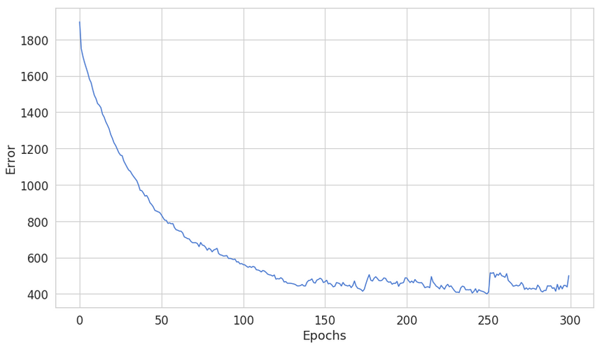
Something looks fishy here, seems like our model can’t continue to reduce the error 150 epochs or so. Let’s have a look at a single prediction:
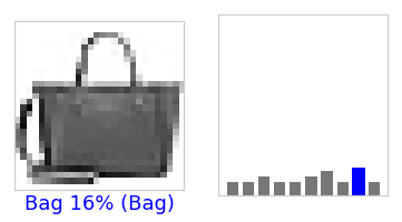
That one seems correct! Let’s have a look at few more:
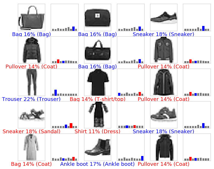
Not too good. How about the training & testing accuracy:
1print('Train Accuracy: %.2f%%' % (nn.score(X_train, y_train) * 100))2print('Test Accuracy: %.2f%%' % (nn.score(X_test, y_test) * 100))1Train Accuracy: 50.13%2Test Accuracy: 49.83%Well, those don’t look that good. While a random classifier will return ~10% accuracy, ~50% accuracy on the test dataset will not make a practical classifier either.
Improving the accuracy
That “jagged” line on the training error chart shows the inability of our model to converge. Recall that we use the Backpropagation algorithm to train our model. Training Neural Nets converge much faster when data is normalized.
We’ll use scikit-learn`s scale to normalize our data. The documentation states that:
Center to the mean and component wise scale to unit variance.
Here is the new training method:
1from sklearn.preprocessing import scale23X_train_scaled = scale(X_train.astype(np.float64))4X_test_scaled = scale(X_test.astype(np.float64))56nn = NNClassifier(7 n_classes=N_CLASSES,8 n_features=N_FEATURES,9 n_hidden_units=50,10 l2=0.5,11 l1=0.0,12 epochs=300,13 learning_rate=0.001,14 n_batches=25,15 random_seed=RANDOM_SEED16).fit(X_train_scaled, y_train);Let’s have a look at the error:
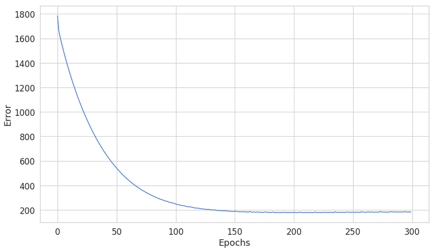
The error seems a lot more stable and settles at lower point - ~200 vs ~400. Let’s have a look at some predictions:
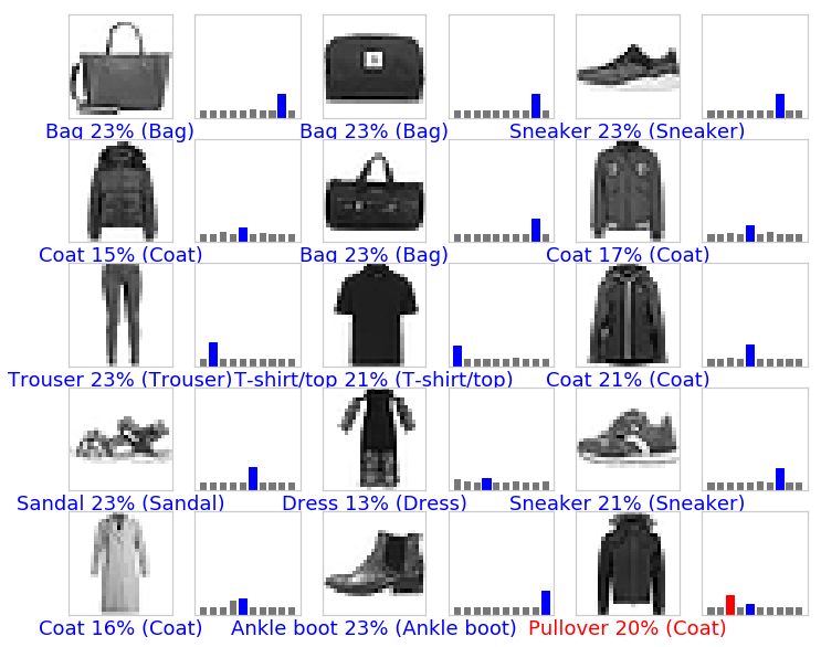
Those look much better, too! Finally, the accuracy:
1print('Train Accuracy: %.2f%%' % (nn.score(X_train_scaled, y_train) * 100))2print('Test Accuracy: %.2f%%' % (nn.score(X_test_scaled, y_test) * 100))1Train Accuracy: 92.13%2Test Accuracy: 87.03%~87% (vs ~50%) on the training set is a vast improvement over the unscaled method. Finally, your hard work paid off!
Conclusion
What a ride! I hope you got a blast working on your first Neural Network from scratch, too!
You learned how to process image data, transform it, and use it to train your Neural Network. We used some handy tricks (scaling) to vastly improve the performance of the classifier.
Share
Want to be a Machine Learning expert?
You'll never get spam from me