TL;DR Learn how to handle underfitting and overfitting models using TensorFlow 2, Keras and scikit-learn. Understand how you can use the bias-variance tradeoff to make better predictions.

The problem of the goodness of fit can be illustrated using the following diagrams:

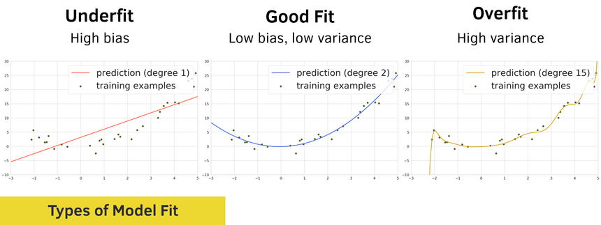
One way to describe the problem of underfitting is by using the concept of bias:

• a model has a high bias if it makes a lot of mistakes on the training data. We also say that the model underfits.

• a model has a low bias if predicts well on the training data

Naturally, we can use another concept to describe the problem of overfitting - variance:

• a model has a high variance if it predicts very well on the training data but performs poorly on the test data. Basically, overfitting means that the model has memorized the training data and can’t generalize to things it hasn’t seen.

• A model has a low variance if it generalizes well on the test data

Getting your model to low bias and low variance can be pretty elusive 🦄. Nonetheless, we’ll try to solve some of the common practical problems using a realistic dataset.

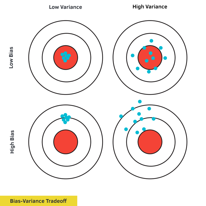
Here’s another way to look at the bias-variance tradeoff (heavily inspired by the original diagram of Andrew Ng):

You’ll learn how to diagnose and fix problems when:

• Your data has no predictive power
• Your model is too simple to make good predictions
• Your data brings the Curse of dimensionality
• Your model is too complex

Run the complete code in your browser

Data

We’ll use the Heart Disease dataset provided by UCI and hosted on Kaggle. Here is the description of the data:

This database contains 76 attributes, but all published experiments refer to using a subset of 14 of them. In particular, the Cleveland database is the only one that has been used by ML researchers to this date. The “goal” field refers to the presence of heart disease in the patient. It is integer valued from 0 (no presence) to 4.

We have 13 features and 303 rows of data. We’re using those to predict whether or not a patient has heart disease.

Let’s start with downloading and loading the data into a Pandas dataframe:

1!pip install tensorflow-gpu
2!pip install gdown
3
4!gdown --id 1rsxu0CKFfI-xR1pH-5JQHcfZ7MIa08Q6 --output heart.csv

1df = pd.read_csv('heart.csv')

Exploration

We’ll have a look at how well balanced the patients with and without heart disease are:

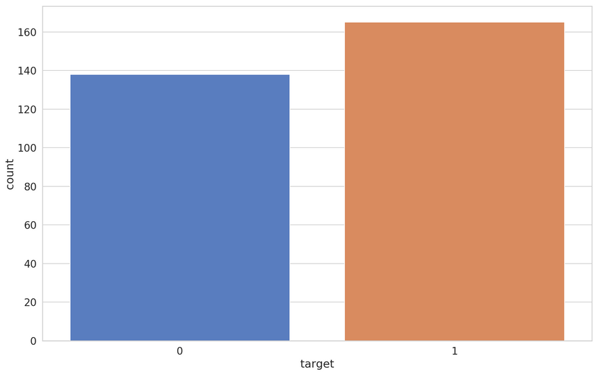
That looks pretty good. Almost no dataset will be perfectly balanced anyways. Do we have missing data?

1df.isnull().values.any()

1false

Nope. Let’s have a look at the correlations between the features:

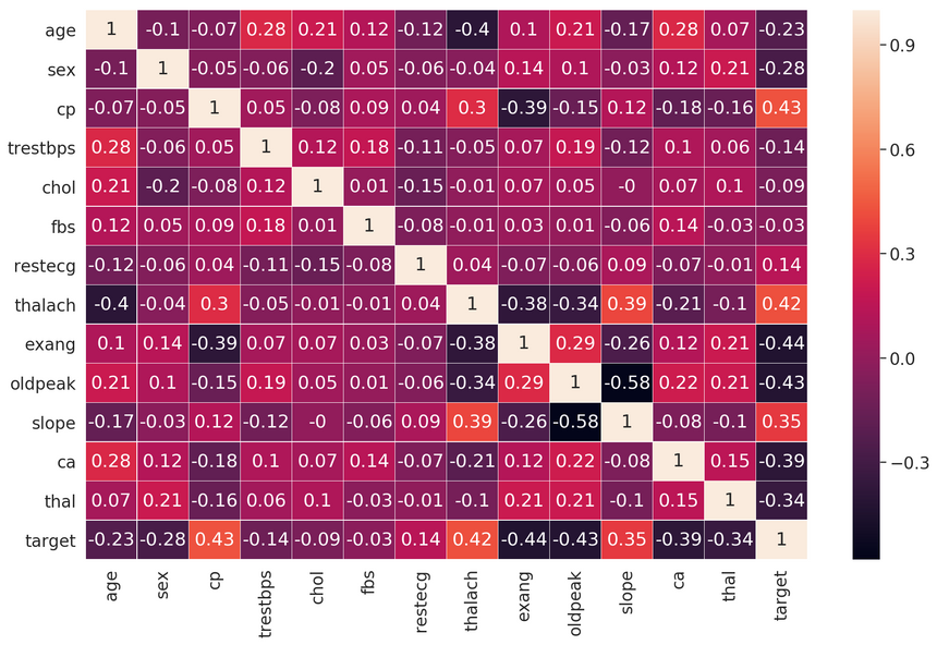
Features like cp (chest pain type), exang (exercise induced angina), and oldpeak (ST depression induced by exercise relative to rest) seem to have a decent correlation with our target variable.

Let’s have a look at the distributions of our features, starting with the most correlated to the target variable:

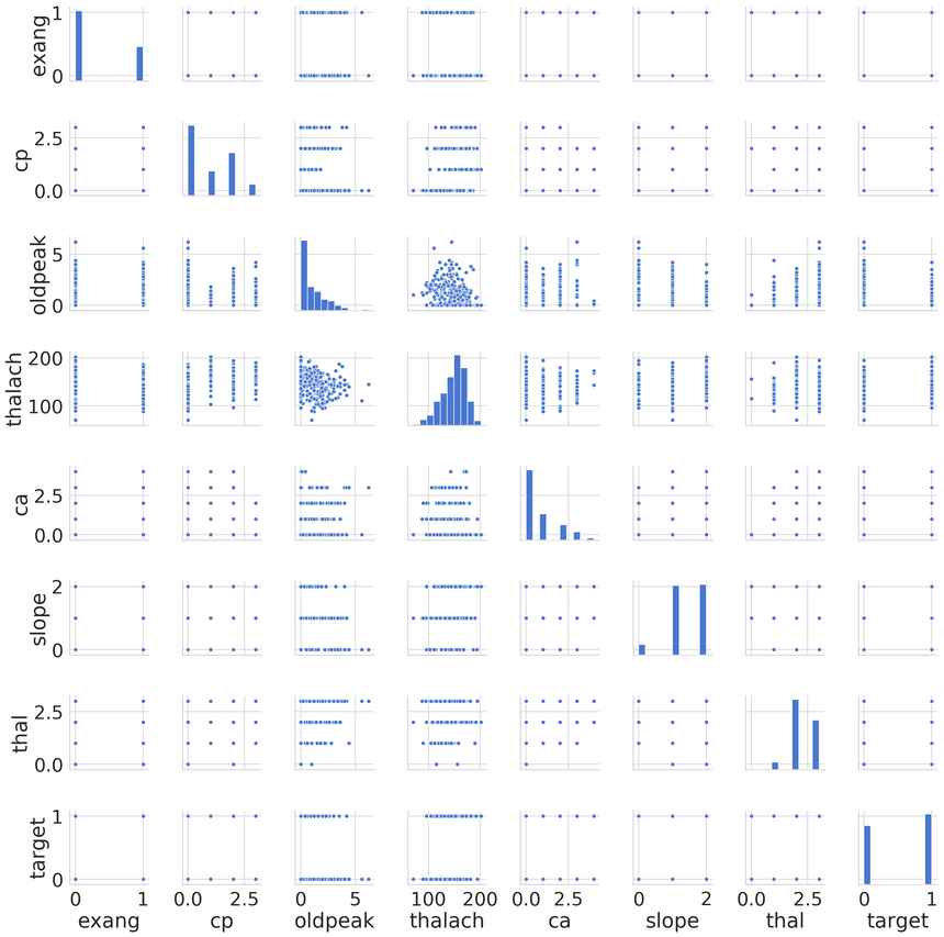
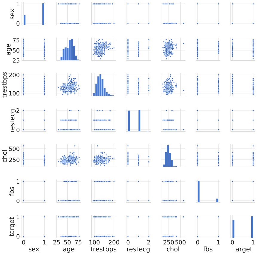
Seems like only oldpeak is a non-categorical feature. It appears that the data contains several features with outliers. You might want to explore those on your own, if interested :)

Underfitting

We’ll start by building a couple of models that underfit and proceed by fixing the issue in some way.

Recall that your model underfits when it makes mistakes on the training data. Here are the most common reasons for that:

• The data features are not informative
• Your model is too simple to predict the data (e.g. linear model predicts non-linear data)

Data with no predictive power

We’ll build a model with the trestbps (resting blood pressure) feature. Its correlation with the target variable is low: -0.14. Let’s prepare the data:

1from sklearn.model_selection import train_test_split
2
3X = df[['trestbps']]
4y = df.target
5
6X_train, X_test, y_train, y_test = \
7 train_test_split(X, y, test_size=0.2, random_state=RANDOM_SEED)

We’ll build a binary classifier with 2 hidden layers:

1def build_classifier(train_data):
2  model = keras.Sequential([
3    keras.layers.Dense(
4      units=32,
5      activation='relu',
6      input_shape=[train_data.shape[1]]
7    ),
8    keras.layers.Dense(units=16, activation='relu'),
9    keras.layers.Dense(units=1),
10  ])
11
12  model.compile(
13    loss="binary_crossentropy",
14    optimizer="adam",
15    metrics=['accuracy']
16  )
17
18  return model

And train it for 100 epochs:

1BATCH_SIZE = 32
2
3clf = build_classifier(X_train)
4
5clf_history = clf.fit(
6  x=X_train,
7  y=y_train,
8  shuffle=True,
9  epochs=100,
10  validation_split=0.2,
11  batch_size=BATCH_SIZE,
12  verbose=0
13)

Here’s how the train and validation accuracy changes during training:

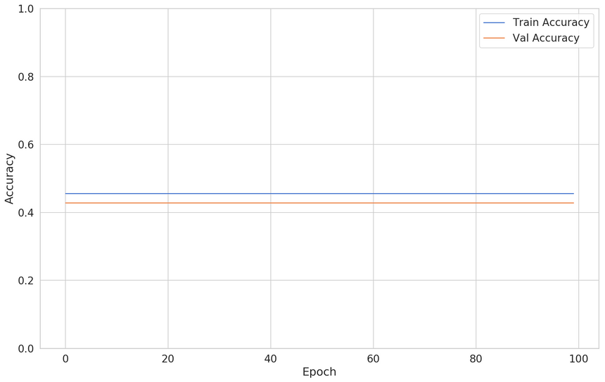
Our model is flatlining. This is expected, the feature we’re using has no predictive power.

The fix

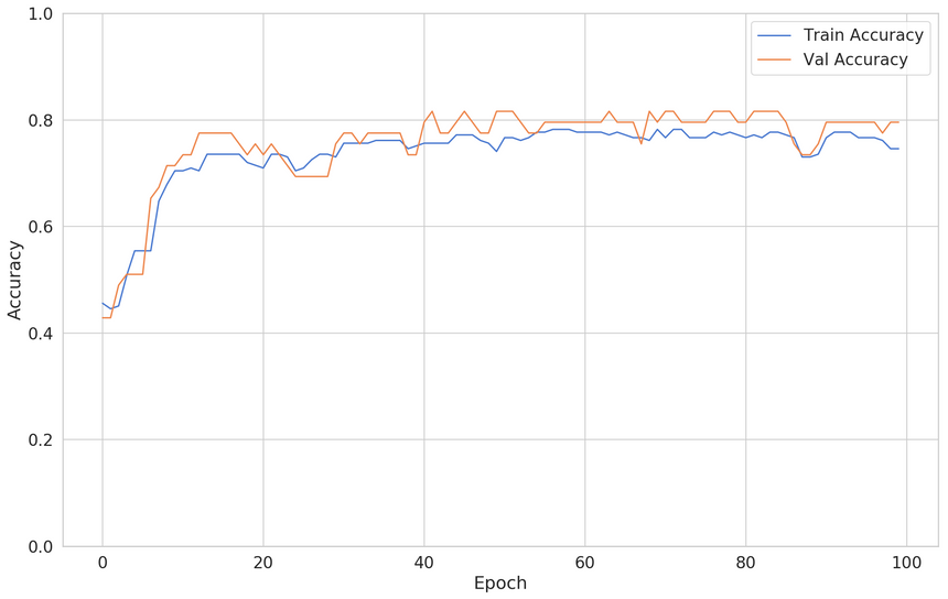
Knowing that we’re using an uninformative feature makes it easy to fix the issue. We can use other feature(s):

1X = pd.get_dummies(df[['oldpeak', 'cp']], columns=["cp"])
2y = df.target
3
4X_train, X_test, y_train, y_test = \
5 train_test_split(X, y, test_size=0.2, random_state=RANDOM_SEED)

And here are the results (using the same model, created from scratch):

Underpowered model

In this case, we’re going to build a regressive model and try to predict the patient maximum heart rate (thalach) from its age.

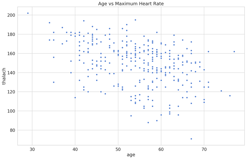
Before starting our analysis, we’ll use MinMaxScaler from scikit-learn to scale the feature values in the 0-1 range:

1from sklearn.preprocessing import MinMaxScaler
2
3s = MinMaxScaler()
4
5X = s.fit_transform(df[['age']])
6y = s.fit_transform(df[['thalach']])
7
8X_train, X_test, y_train, y_test = \
9 train_test_split(X, y, test_size=0.2, random_state=RANDOM_SEED)

Our model is a simple linear regression:

1lin_reg = keras.Sequential([
2  keras.layers.Dense(
3    units=1,
4    activation='linear',
5    input_shape=[X_train.shape[1]]
6  ),
7])
8
9lin_reg.compile(
10  loss="mse",
11  optimizer="adam",
12  metrics=['mse']
13)

Here’s the train/validation loss:

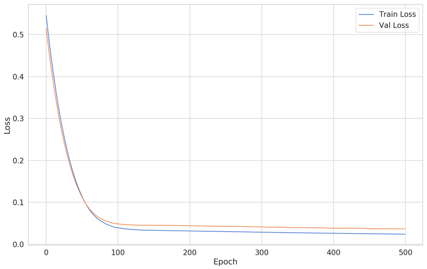
Here are the predictions from our model:

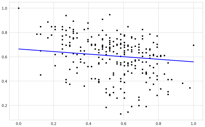
You can kinda see that a linear model might not be the perfect fit here.

The fix

We’ll use the same training process, except that our model is going to be a lot more complex:

1lin_reg = keras.Sequential([
2  keras.layers.Dense(
3    units=64,
4    activation='relu',
5    input_shape=[X_train.shape[1]]
6  ),
7  keras.layers.Dropout(rate=0.2),
8  keras.layers.Dense(units=32, activation='relu'),
9  keras.layers.Dropout(rate=0.2),
10  keras.layers.Dense(units=16, activation='relu'),
11  keras.layers.Dense(units=1, activation='linear'),
12])
13
14lin_reg.compile(
15  loss="mse",
16  optimizer="adam",
17  metrics=['mse']
18)

Here’s the training/validation loss:

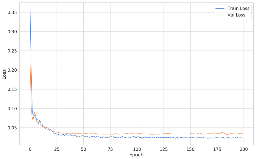
Our validation loss is similar. What about the predictions:

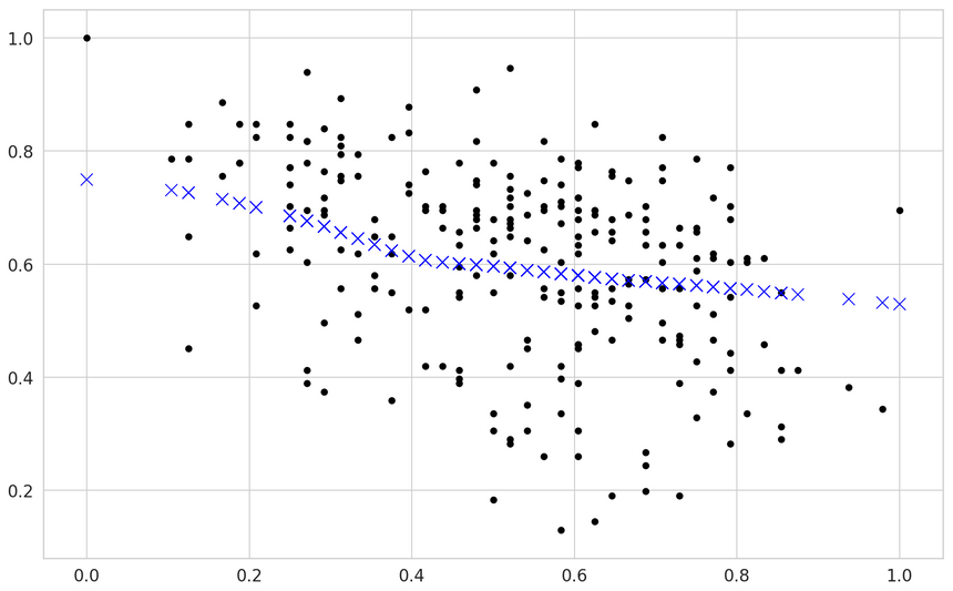
Interesting, right? Our model broke from the linear-only predictions. Note that this fix included adding more parameters and increasing the regularization (using Dropout).

Overfitting

A model overfits when predicts training data well but performs poor on the validation set. Here are some of the reasons for that:

• Your data has many features but a small number of examples (curse of dimensionality)
• Your model is too complex for the data (Early stopping)

Curse of dimensionality

The Curse of dimensionality refers to the problem of having too many features (dimensions), compared to the data points (examples). The most common way to solve this problem is to add more information.

We’ll use a couple of features to create our dataset:

1X = df[['oldpeak', 'age', 'exang', 'ca', 'thalach']]
2X = pd.get_dummies(X, columns=['exang', 'ca', 'thalach'])
3y = df.target
4
5X_train, X_test, y_train, y_test = \
6  train_test_split(X, y, test_size=0.2, random_state=RANDOM_SEED)

Our model contains one hidden layer:

1def build_classifier():
2
3  model = keras.Sequential([
4    keras.layers.Dense(
5      units=16,
6      activation='relu',
7      input_shape=[X_train.shape[1]]
8    ),
9    keras.layers.Dense(units=1, activation='sigmoid'),
10  ])
11
12  model.compile(
13    loss="binary_crossentropy",
14    optimizer="adam",
15    metrics=['accuracy']
16  )
17
18  return model

Here’s the interesting part. We’re using just a tiny bit of the data for training:

1clf = build_classifier()
2
3clf_history = clf.fit(
4  x=X_train,
5  y=y_train,
6  shuffle=True,
7  epochs=500,
8  validation_split=0.95,
9  batch_size=BATCH_SIZE,
10  verbose=0
11)

Here’s the result of the training:

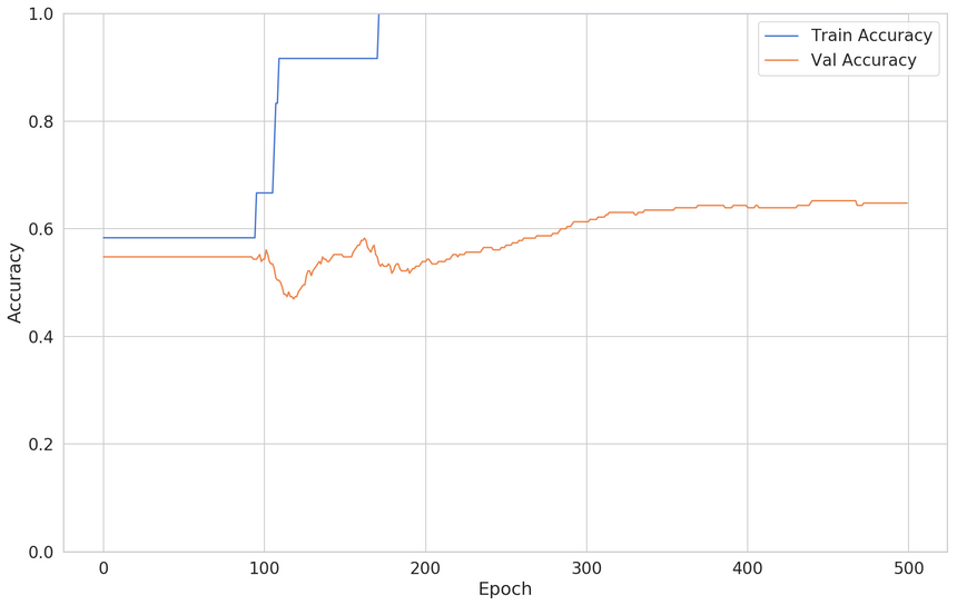
The fix

Our solution will be pretty simple - add more data. However, you can provide additional information via other methods (i.e. Bayesian prior) or reduce the number of features via feature selection.

Let’s try the simple approach:

1clf = build_classifier()
2
3clf_history = clf.fit(
4  x=X_train,
5  y=y_train,
6  shuffle=True,
7  epochs=500,
8  validation_split=0.2,
9  batch_size=BATCH_SIZE,
10  verbose=0
11)

The training/validation loss looks like this:

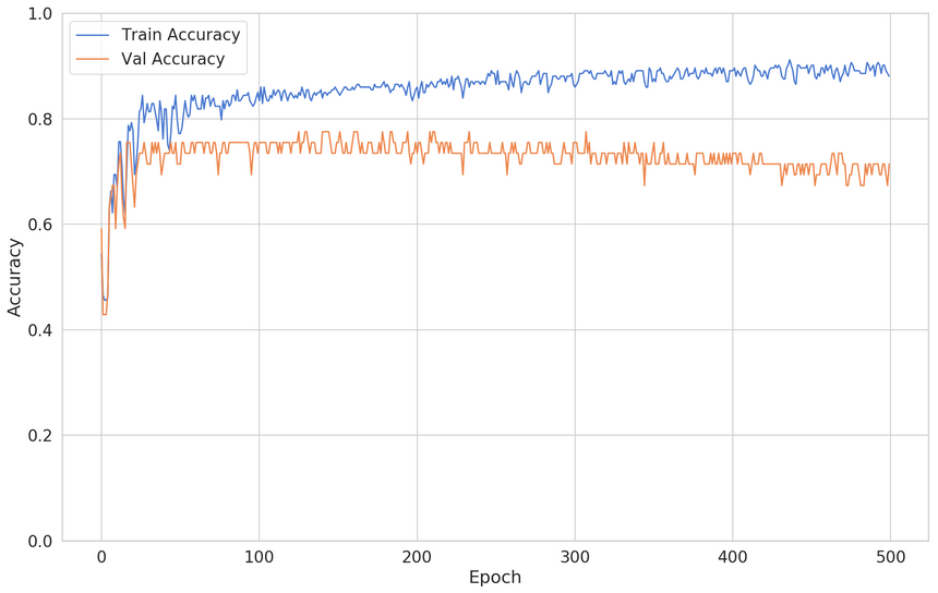
While this is an improvement, you can see that the validation loss starts to decrease after some time. How can you fix this?

Too complex model

We’ll reuse the dataset but build a new model:

1def build_classifier():
2  model = keras.Sequential([
3    keras.layers.Dense(
4      units=128,
5      activation='relu',
6      input_shape=[X_train.shape[1]]
7    ),
8    keras.layers.Dense(units=64, activation='relu'),
9    keras.layers.Dense(units=32, activation='relu'),
10    keras.layers.Dense(units=16, activation='relu'),
11    keras.layers.Dense(units=8, activation='relu'),
12    keras.layers.Dense(units=1, activation='sigmoid'),
13  ])
14
15  model.compile(
16    loss="binary_crossentropy",
17    optimizer="adam",
18    metrics=['accuracy']
19  )
20
21  return model

Here is the result:

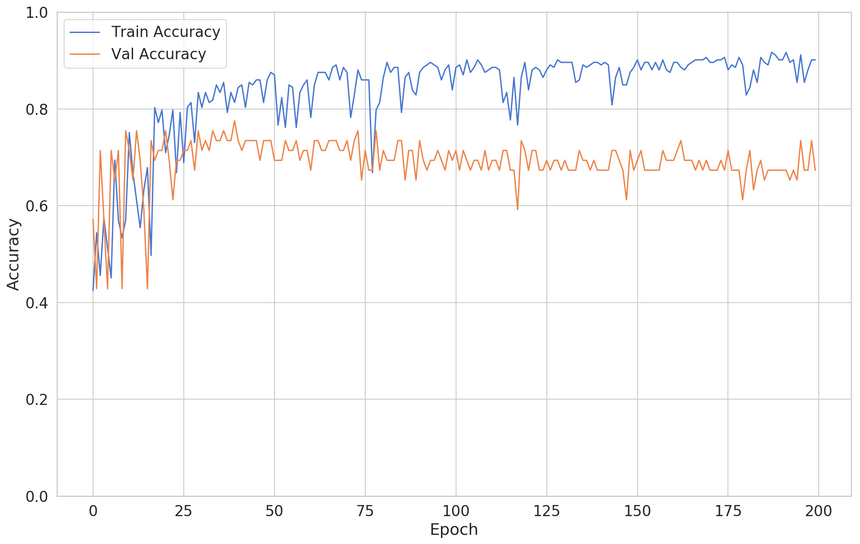
You can see that the validation accuracy starts to decrease after epoch 25 or so.

The Fix #1

One way to fix this would be to simplify the model. But what if you spent so much time fine-tuning it? You can see that your model is performing better at a previous stage of the training.

You can use the EarlyStopping callback to stop the training at some point:

1clf = build_classifier()
2
3early_stop = keras.callbacks.EarlyStopping(
4  monitor='val_accuracy',
5  patience=25
6)
7
8clf_history = clf.fit(
9  x=X_train,
10  y=y_train,
11  shuffle=True,
12  epochs=200,
13  validation_split=0.2,
14  batch_size=BATCH_SIZE,
15  verbose=0,
16  callbacks=[early_stop]
17)

Here’s the new training/validation loss:

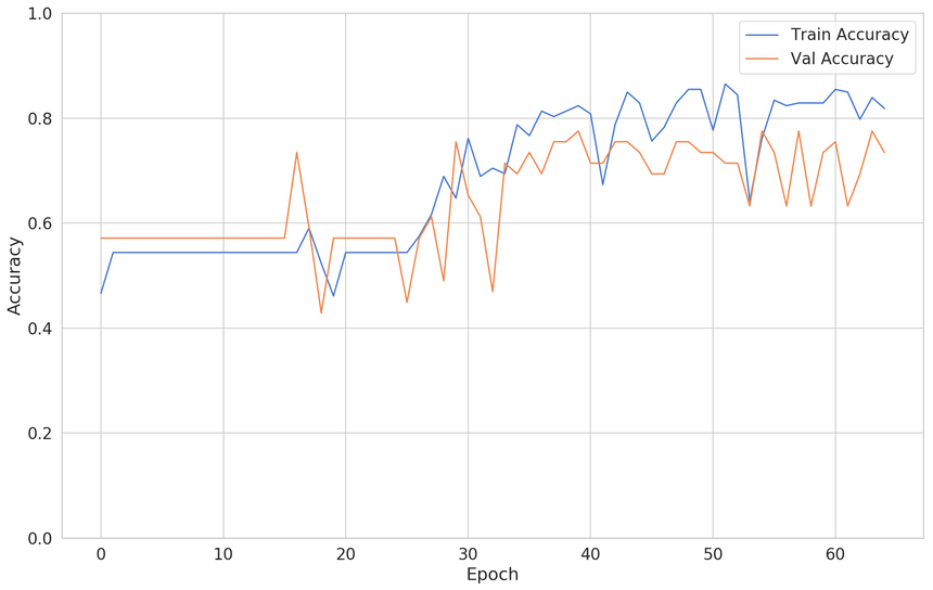
Alright, looks like the training stopped much earlier than epoch 200. Faster training and a more accurate model. Nice!

The Fix #2

Another approach to fixing this problem is by using Regularization. Regularization is a set of methods that forces the building of a less complex model. Usually, you get higher bias (less correct predictions on the training data) but reduced variance (higher accuracy on the validation dataset).

One of the most common ways to Regularize Neural Networks is by using Dropout.

Dropout is a regularization technique for reducing overfitting in neural networks by preventing complex co-adaptations on training data. It is a very efficient way of performing model averaging with neural networks. The term “dropout” refers to dropping out units (both hidden and visible) in a neural network.

Using Dropout in Keras is really easy:

1model = keras.Sequential([
2    keras.layers.Dense(
3      units=128,
4      activation='relu',
5      input_shape=[X_train.shape[1]]
6    ),
7    keras.layers.Dropout(rate=0.2),
8    keras.layers.Dense(units=64, activation='relu'),
9    keras.layers.Dropout(rate=0.2),
10    keras.layers.Dense(units=32, activation='relu'),
11    keras.layers.Dropout(rate=0.2),
12    keras.layers.Dense(units=16, activation='relu'),
13    keras.layers.Dropout(rate=0.2),
14    keras.layers.Dense(units=8, activation='relu'),
15    keras.layers.Dense(units=1, activation='sigmoid'),
16  ])
17
18model.compile(
19  loss="binary_crossentropy",
20  optimizer="adam",
21  metrics=['accuracy']
22)

Here’s how the training process has changed:

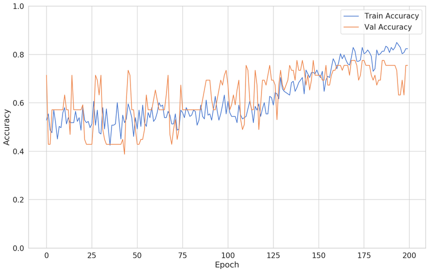
The validation accuracy seems very good. Note that the training accuracy is down (we have a higher bias). There you have it, two ways to solve one issue!

Conclusion

Well done! You now have the toolset for dealing with the most common problems related to high bias or high variance. Here’s a summary:

• Your data has no predictive power - use different data
• Your model is too simple to make good predictions - use model with more parameters
• Your data brings the Curse of dimensionality - use more data, reduce the number of features or use Bayesian Prior to provide more information
• Your model is too complex - use Early Stopping or Regularization to force creating a simpler model

Run the complete code in your browser

References

• Bias-Variance Tradeoff in Machine Learning

• Bias–variance tradeoff

• Diagnosing Bias vs. Variance

• What is the curse of dimensionality?