TL;DR Overview of fundamental classification and regression learning algorithms. Learn when should you use each and what data preprocessing is required. Each algorithm is presented along with an example done in scikit-learn.

This guide explores different supervised learning algorithms, sorted by increasing complexity (measured by the number of model parameters and hyperparameters). I would strongly suggest you start with the simpler ones when working on a new project/problem.

But why not just use Deep Neural Networks for everything? You can, and maybe you should. But simplicity can go a long way before the need for ramping up the complexity in your project. It is also entirely possible to not be able to tune your Neural Net to beat some of the algorithms described here.

You’re going to learn about:

• Linear Regression
• Logistic Regression
• k-Nearest Neighbors
• Naive Bayes
• Decision Trees
• Support Vector Machines

Run the complete notebook in your browser

The complete project on GitHub

What Makes a Learning Algorithm?

In their essence, supervised Machine Learning algorithms learn a mapping function $f$ that maps the data features $X$ to labels $y$. The goal is to make the mapping as accurate as possible. We can define the problem as:

where $e$ is an irreducible error. That error is independent of the data and can’t be lowered using the data (hence the name).

The problem of finding the function $f$ is notoriously difficult. In practice, you’ll be content with a good approximation. There are many ways to get the job done. What do they have in common?

Components of a Learning Algorithm

• Loss functions
• Optimizer that tries to minimize the loss function

The Loss Function outputs a numerical value that shows how “bad” your model predictions are. The closer the value is to 0, the better the predictions.

The optimizer’s job is to find the best possible values for the model parameters that minimize the loss function. This is done with the help of the training data and an algorithm that searches for the parameter values.

Gradient Descent is the most commonly used algorithm for optimization. It finds a local minimum of a function by starting at a random point and takes steps in a direction and size given by the gradient.

Our Data

We’ll use the Auto Data Set to create examples for various classification and regression algorithms.

Gas mileage, horsepower, and other information for 392 vehicles. This dataset was taken from the StatLib library which is maintained at Carnegie Mellon University. The dataset was used in the 1983 American Statistical Association Exposition.

Let’s download the data and load it into a Pandas data frame:

1!gdown --id 16VDAc-x1fGa2lpsI8xtLHK6z_3m36JBx --output auto.csv

1auto_df = pd.read_csv("auto.csv", index_col=0)
2auto_df.shape

1(392, 9)

We have 392 vehicles and we’ll use this subset of the features:

• mpg - miles per gallon

• horsepower - Engine horsepower

• weight - Vehicle weight (lbs.)

• acceleration - Time to accelerate from 0 to 60 mph (sec.)

• origin - Origin of car (1. American, 2. European, 3. Japanese)

We have no missing data.

Data Preprocessing

We’re going to define two helper functions that prepare a classification and a regression dataset based on our data. But first, we’re going to add a new feature that specifies whether a car is American made or not:

1auto_df['is_american'] = (auto_df.origin == 1).astype(int)

We’re going to use the StandarScaler to scale our datasets:

1from sklearn.preprocessing import StandardScaler
2
3def create_regression_dataset(
4    df,
5    columns=['mpg', 'weight', 'horsepower']
6):
7
8  all_columns = columns.copy()
9  all_columns.append('acceleration')
10
11  reg_df = df[all_columns]
12  reg_df = StandardScaler().fit_transform(reg_df[all_columns])
13  reg_df = pd.DataFrame(reg_df, columns=all_columns)
14
15  return reg_df[columns], reg_df.acceleration
16
17def create_classification_dataset(df):
18  columns = ['mpg', 'weight', 'horsepower']
19
20  X = df[columns]
21  X = StandardScaler().fit_transform(X)
22  X = pd.DataFrame(X, columns=columns)
23
24  return X, df.is_american

Evaluation

We’re going to use k-fold cross validation to evaluate the performance of our models. Note that this guide is NOT benchmarking model performance. Here are the definitions of our evaluation functions:

1from sklearn.model_selection import KFold, cross_val_score
2
3def eval_model(model, X, y, score):
4  cv = KFold(n_splits=10, random_state=RANDOM_SEED)
5  results = cross_val_score(model, X, y, cv=cv, scoring=score)
6  return np.abs(results.mean())
7
8def eval_classifier(model, X, y):
9  return eval_model(model, X, y, score="accuracy")
10
11def eval_regressor(model, X, y):
12  return eval_model(model, X, y, score="neg_mean_squared_error")

We are using accuracy (percent of correctly predicted examples) as a metric for our classification examples and mean squared error (explained below) for the regression examples.

Linear Regression

Linear Regression tries to build a line that can best describe the relationship between two variables $X$ and $Y$. That line is called “best-fit” and is closest to the points $(x_i, y_i)$.

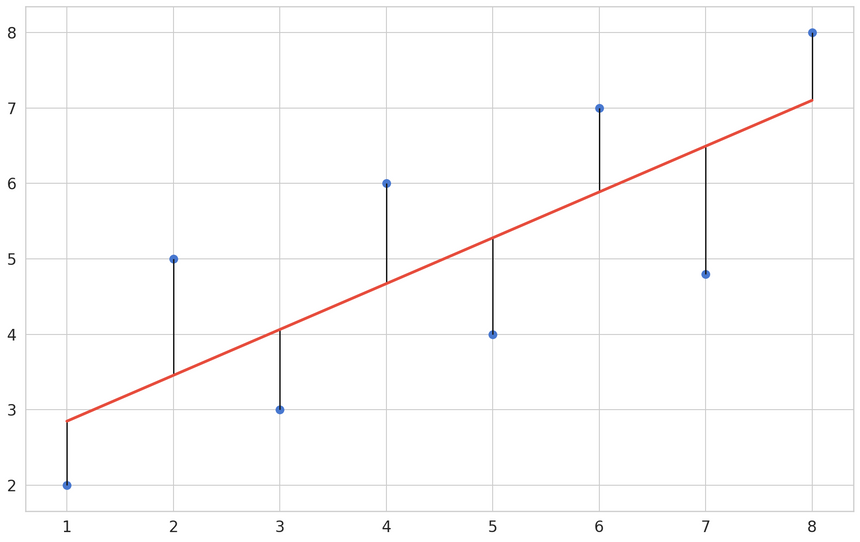
$Y$ is known as the dependent variable and it is continious - e.g. number of sales, price, weight. This is the variable which values we’re trying to predict. $X$ is known as explanatory (or independent) variable. We use this variable to predict the value of $Y$. Note that we’re assuming a linear relationship between the variables.

Definition

Our dataset consists of $m$ labeled examples $(x_i, y_i)$, where $x_i$ is $D$-dimensional feature vector, $y_i \in \mathbb{R}$ and every feature $x_i^j \in \mathbb{R}, j = 1, \ldots, D$. We want to build a model that predicts unknown $y$ for a given $x$. Our model is defined as:

where $w$ and $b$ are parameters of our model that we’ll learn from the data. $w$ defines the slope of the model, while $b$ defines the intercept point with the vertical axis.

Making Predictions

Linear regression that makes the most accurate prediction has optimal values for the parameters $w$ and $b$. Let’s denote those as $w^*$ and $b^*$. How can we find those values?

We’ll use an objective metric that tells us how good the current values are. *Optimal parameter values will minimize that metric.

The most used metric in such cases is Mean Squared Error(MSE). It is defined as:

The MSE measures how much the average model predictions vary from the correct values. The number is higher when the model is making “bad” predictions. Model that makes perfect predictions has a MSE of 0.

We’ve transformed the problem of finding optimal values for our parameters to minimizing MSE. We can do that using an optimization algorithm known as Stochastic Gradient Descent.

Simple Linear Regression

This type of Linear Regression uses a single feature to predict the target variable. Let’s use the horsepower to predict car acceleration:

1from sklearn.linear_model import LinearRegression
2
3X, y = create_regression_dataset(auto_df, columns=['horsepower'])
4
5reg = LinearRegression()
6eval_regressor(reg, X, y)

10.5283214994429212

Multiple Linear Regression

Of course, we can use more features to predict the acceleration. This is called Multiple Linear Regression. The training process looks identical (thanks to the nice interface that scikit-learn provides):

1X, y = create_regression_dataset(auto_df)
2
3reg = LinearRegression()
4eval_regressor(reg, X, y)

10.4351523357394419

The $R^2$ score has increased. Can we do better? How?

Ridge Regression

1from sklearn.linear_model import Ridge
2
3X, y = create_regression_dataset(auto_df)
4
5reg = Ridge(alpha=0.0005, random_state=RANDOM_SEED)
6
7eval_regressor(reg, X, y)

10.4351510356810997

When To Use Linear Regression?

Start with this algorithm when starting a regression problem. Useful when your features can be separated by a straight line.

Pros:

• Fast to train on large datasets
• Fast inference time
• Easy to understand/interpret the results

Cons:

• Need to scale numerical features
• Preprocess categorical data
• Can predict only linear relationships

Logistic Regression

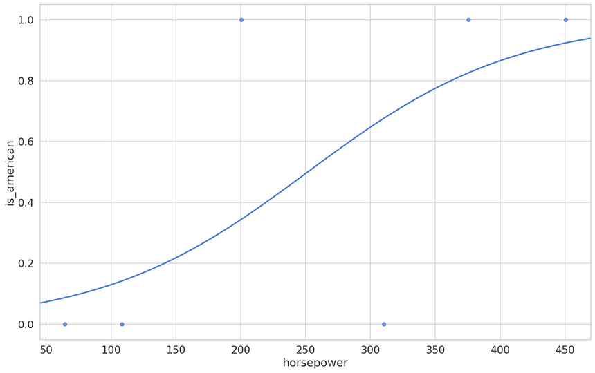
Logistic Regression has a similar formulation to Linear Regression (hence the name) but allows you to solve classification problems. The most common problem solved in practice is binary classification, so we’ll discuss this application in particular.

Making Predictions

We already have a way to make predictions with Linear Regression. The problem is that they are in $(-\infty, +\infty)$ interval. How can you use that to make true/false predictions?

If we map false to 0 and true to 1, we can use the Sigmoid function to bound the domain to $(0, 1)$. It is defined by:

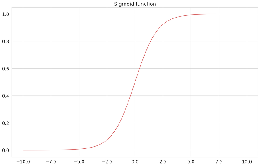
We can use the Sigmoid function and a predefined threshold ( commonly set to 0.5) to map values larger than the threshold to a positive label; otherwise, it’s negative.

Combining the Linear Regression equation with the Sigmoid function gives us:

Your next task is to find optimal parameter values for $w^*$ and $b^*$. We can use the Log Loss to measure how good our classifications are:

Our goal is to minimize the loss value. So, a value close to 0 says that the classifier is very good at predicting on the dataset.

Logg Loss requires that your classifier outputs probability for each possible class, instead of just the most likely one. Ideal classifier assigns a probability equal to 1 for the correct class and 0 for all else.

Just as with Linear Regression, we can use Gradient Descent to find the optimal parameters for our model. How can we do it with scikit-learn?

Example

The LogisticRegression from scikit-learn allows you to do multiclass classification. It also applies $l2$ regularization by default. Let’s use it to predict car model origin:

1from sklearn.linear_model import LogisticRegression
2
3X, y = create_classification_dataset(auto_df)
4
5clf = LogisticRegression(solver="lbfgs")
6eval_classifier(clf, X, y)

10.787948717948718

We got about ~79% accuracy, which is quite good, considering how simple the model is.

When To Use It?

Logistic Regression should be your first choice when solving a new classification problem.

Pros:

• Easy to understand and interpret
• Easy to configure (small number of hyperparameters)
• Outputs the likelihood for each class

Cons:

• Requires data scaling
• Assumes linear relationship in the data
• Sensitive to outliers

k-Nearest Neighbors

During training, this algorithm stores the data in some sort of efficient data structure (like k-d tree), so it is available for later. Predictions are made by finding $k$ (hence the name) similar training examples and returning the most common label (in case of classification) or avering label values (in case of regression). How do we measure similarity?

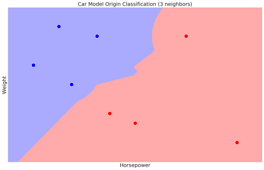
Measuring the similarity of two data points is most commonly done by measuring the distance between them. Some of the most popular distance measures are Euclidean Distance:

measures the straight-line distance between two points in Euclidean space

and Cosine Similarity:

which measures how similar the directions of two vectors are.

You might think that normalizing features is really important for this algorithm, and you’ll be right!

Example

k-Nearest Neighbors (KNN) can be used for classification and regression tasks. KNeighborsClassifier offers a nice set of options for parameters like - number of neighbors and the type of metric to use. Let’s look at an example:

1from sklearn.neighbors import KNeighborsClassifier
2
3X, y = create_classification_dataset(auto_df)
4
5clf = KNeighborsClassifier(n_neighbors=24)
6eval_classifier(clf, X, y)

10.8008333333333335

How can you find good values for $k$ (number of neighbors)? Usually, you just try a lot of different values.

When To Use It?

This algorithm might have very good performance when compared to Linear Regression. It works quite well on smallish datasets with not that many features.

Pros:

• Easy to understand and reason about
• Trains instantly (all of the work is done when predicting data)
• Makes no assumption about input data distributions
• Automatically adjusts predictions as new data comes in

Cons:

• Need to scale numerical features (depends on distance measurements)
• Slow inference time (all of the work is done when predicting data)
• Sensitive to imbalanced datasets - values occuring more often will bias the results. You can use resampling techniques for this issue.
• High dimensional features may produce closeness to many data points. You can apply dimensionality reduction techniques for this issue.

Naive Bayes

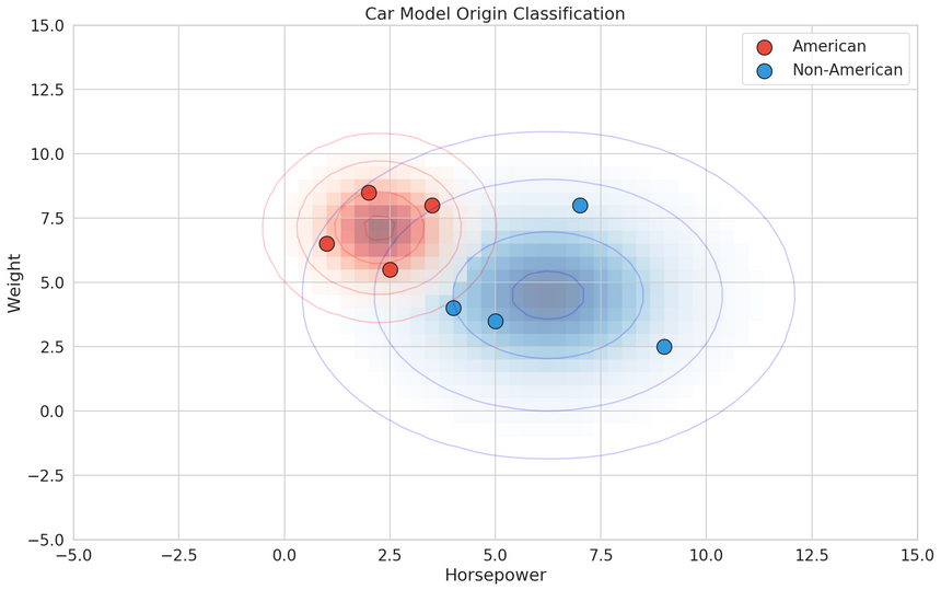
Naive Bayes algorithms calculate the likelihood of each class is correct. They apply Bayes’ theorem to classification problems. That is, with a strong (and often unrealistic) assumption of independence between the features.

Bayes Theorem

Bayes theorem gives the following relationship between the labels and features:

Using the independence assumption we get:

$P({\rm x_1,\ldots,x_n})$ is a normalizing term (constant). We can drop it, since we’re interested in the most probable hypothesis, and use the following classification rule:

Example

Scikit-learn implements multiple Naive Bayes classifiers. We’re going to use GaussianNB which assumes Gaussian distribution of the data:

1from sklearn.naive_bayes import GaussianNB
2
3X, y = create_classification_dataset(auto_df)
4
5clf = GaussianNB()
6eval_classifier(clf, X, y)

10.7597435897435898

When To Use It?

Naive Bayes classifiers are a very good choice for building baseline models that have a probabilistic interpretation of its outputs. Training and prediction speed are very good on large amounts of data.

Pros:

• Fast training and inference performance
• Can be easily interpreted due to probabilistic predictions
• Easy to tune (a few hyperparameters)
• No feature scaling required
• Can handle imbalanced datasets - with Complement Naive Bayes

Cons:

• Naive assumption about independence, which is rarely true (duh)
• Performance suffers when multicollinearity is present

Decision Trees

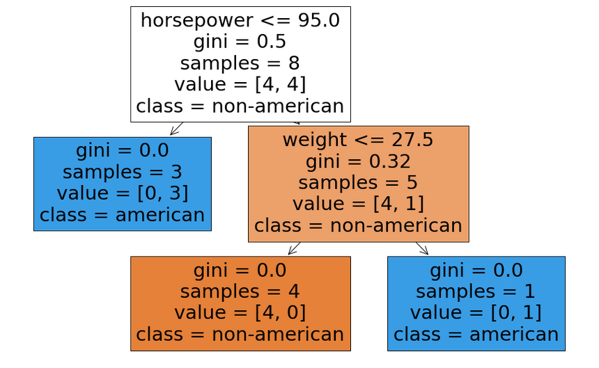
Decision Tree algorithms build (mostly binary) trees using the data to choose split points. At each node, a specific feature is examined and compared to a threshold. We go to the left if the value is below the threshold, else we go right. We get an answer (prediction) of the model when a leaf node is reached.

Example

Scikit-learn offers multiple tree-based algorithms for both regression and classification. Let’s look at an example:

1from sklearn.tree import DecisionTreeRegressor
2
3X, y = create_regression_dataset(auto_df)
4
5reg = DecisionTreeRegressor()
6eval_regressor(reg, X, y)

10.6529188972733717

Random Forests

The Random Forest algorithm combines multiple decision trees. Each tree is trained on a random subset of the data and has a low bias (low error on the training data) and high variance (high error on the test data). Aggregating the trees allows you to build a model with low variance.

1from sklearn.ensemble import RandomForestRegressor
2
3X, y = create_regression_dataset(auto_df)
4
5reg = RandomForestRegressor(n_estimators=50)
6eval_regressor(reg, X, y)

10.3976871715935767

Note the error difference between a single Decision Tree and a Random Forest with 50 weak Decision Trees.

Boosting

This method builds multiple decision trees iteratively. Each new tree tries to fix the errors made by the previous one. At each step, the error between the predicted and actual data is added to the loss and then minimized at the next step.

1from sklearn.ensemble import GradientBoostingRegressor
2
3X, y = create_regression_dataset(auto_df)
4
5reg = GradientBoostingRegressor(n_estimators=100)
6eval_regressor(reg, X, y)

10.37605497373246266

Now go to Kaggle and check how many competitions are won by using this method.

When To Use It?

In practice, you’ll never be using a single Decision Tree. Ensemble methods (multiple decision trees) are the way to go. Overall, boosting can give you the best possible results (especially when using libraries like LightGBM). But you have a lot of hyperparameters to tune. It might take a lot of time and experience to develop really good models.

Pros:

• Easy to interpret and visualize (white box models)
• Can handle numerical and categorical data
• No complex data preprocessing - no normalization or missing data imputation is need
• Fast prediction speed - O(log n)
• Can be used in ensembles to prevent overfitting and increase accuracy
• Perform very well on both regression and classification tasks
• Show feature importances

Cons:

• Do not work well with imbalanced datasets - fixed by balancing or providing class weights
• Easy to overfit - you can build very deep trees that memorize every feature value - fixed by limiting tree depth
• Must be used in ensembles to get good results in practice
• Sensitive to data changes (small variation can build entirely different tree) - fixed using ensembles

Support Vector Machines (SVM)

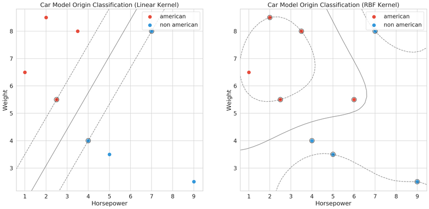
SVM models try to build hyperplanes (n-dimensional lines) that best separate the data. Hyperplanes are created such that there is a maximum distance between the closest example of each class.

Hard-margin

Hard-margin SVMs work when the data is linearly separable. We want to minimize the margin between the support vectors $\Vert w \Vert$ (the closest data points to the separating hyperplane). We have:

satisfying the constraint:

What about data points that cannot be linearly separated?

Soft-margin

In practice, the expectation that the data is linearly separable is unrealistic. We can cut some slack to our SVM and introduce a constant $C$. It determines the tradeoff between increasing the decision boundary and placing each data point on the correct side of the decision boundary.

We want to minimize the following function:

Choosing the correct $C$ is done experimentally. You can look at this parameter as a way to control the bias-variance tradeoff for your model.

Example

Using SVMs on regression problems can be done using the SVR model:

1from sklearn.svm import SVR
2
3X, y = create_regression_dataset(auto_df)
4
5reg = SVR(gamma="auto", kernel="rbf", C=4.5)
6eval_regressor(reg, X, y)

10.32820308689067834

When To Use It?

Support Vector Machines can give you great performance but need careful tuning. You can solve non-linearly separable problems with a proper choice of a kernel function.

Pros:

• Can provide very good results used for regression and classification
• Can learn non-linear boundaries (see the kernel trick)
• Robust to overfitting in higher dimensional space

Cons:

• Large number of hyperparameters
• Data must be scaled
• Data must be balanced
• Sensitive to outliers - can be mitigated by using soft-margin

Conclusion

You covered some of the most used Machine Learning algorithms. But you’ve just scratched the surface. Devil is in the details, and those algorithms have a lot of details surrounding them.

You learned about:

• Linear Regression
• Logistic Regression
• k-Nearest Neighbors
• Naive Bayes
• Decision Trees
• Support Vector Machines

I find it fascinating that there are no clear winners when it comes to having an all-around best algorithm. Your project/problem will inevitably require some careful experimentation and planning. Enjoy the process :)

Run the complete notebook in your browser

The complete project on GitHub

References

• Machine Learning Notation
• Making Sense of Logarithmic Loss
• In Depth: Naive Bayes Classification