TL;DR Learn how to create new examples for your dataset using image augmentation techniques. Load a scanned document image and apply various augmentations. Create an augmented dataset for Object Detection.

Your Deep Learning models are dumb. Detecting objects in a slightly different image, compared to the training examples, can produce hugely incorrect predictions. How can you fix that?

Ideally, you would go and get more training data, and then some more. The more diverse the examples, the better. Except, getting new data can be hard, expensive, or just impossible. What can you do?

You can use your own “creativity” and create new images from the existing ones. The goal is to create transformations that resemble real examples not found in the data.

We’re going to have a look at “basic” image augmentation techniques. Advanced methods like Neural Style Transfer and GAN data augmentation may provide even more performance improvements, but are not covered here.

You’ll learn how to:

• Load images using OpenCV
• Apply various image augmentations
• Compose complex augmentations to simulate real-world data
• Create augmented dataset ready to use for Object Detection

Run the complete notebook in your browser

The complete project on GitHub

Tools for Image Augmentation

Image augmentation is widely used in practice. Your favorite Deep Learning library probably offers some tools for it.

TensorFlow 2 (Keras) gives the ImageDataGenerator. PyTorch offers a much better interface via Torchvision Transforms. Yet, image augmentation is a preprocessing step (you are preparing your dataset for training). Experimenting with different models and frameworks means that you’ll have to switch a lot of code around.

Luckily, Albumentations offers a clean and easy to use API. It is independent of other Deep Learning libraries and quite fast. Also, it gives you a large number of useful transforms.

How can we use it to transform some images?

Augmenting Scanned Documents

Here is the sample scanned document, that we’ll transform using Albumentations:

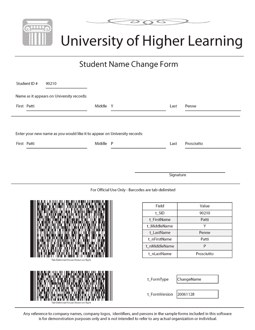
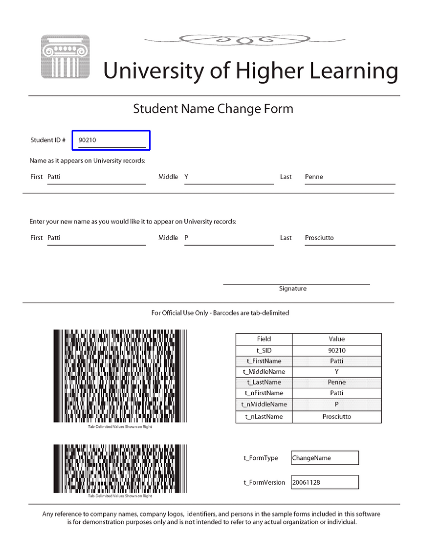
Let’s say that you were tasked with the extraction of the Student Id from scanned documents. One way to approach the problem is to first detect the region that contains the student id and then use OCR to extract the value.

Here is the training example for our Object Detection algorithm:

Let’s start with some basic transforms. But first, let’s create some helper functions that show the augmented results:

1def show_augmented(augmentation, image, bbox):
2  augmented = augmentation(image=image, bboxes=[bbox], field_id=['1'])
3  show_image(augmented['image'], augmented['bboxes'][0])

show_augmented() applies the augmentation on the image and show the result along with the modified bounding box (courtesy of Albumentations). Here is the definition of show_image():

1def show_image(image, bbox):
2  image = visualize_bbox(image.copy(), bbox)
3  f = plt.figure(figsize=(18, 12))
4  plt.imshow(
5    cv2.cvtColor(image, cv2.COLOR_BGR2RGB),
6    interpolation='nearest'
7  )
8  plt.axis('off')
9  f.tight_layout()
10  plt.show()

We start by drawing the bounding box on top of the image and showing the result. Note that OpenCV2 uses a different channel ordering than the standard RGB. We take care of that, too.

Finally, the definition of visualize_bbox():

1BOX_COLOR = (255, 0, 0)
2
3def visualize_bbox(img, bbox, color=BOX_COLOR, thickness=2):
4    x_min, y_min, x_max, y_max = map(lambda v: int(v), bbox)
5
6    cv2.rectangle(
7      img,
8      (x_min, y_min),
9      (x_max, y_max),
10      color=color,
11      thickness=thickness
12    )
13    return img

Bounding boxes are just rectangles drawn on top of the image. We use OpenCV’s rectangle() function and specify the top-left and bottom-right points.

Augmenting bounding boxes requires a specification of the coordinates format:

1# [x_min, y_min, x_max, y_max], e.g. [97, 12, 247, 212].
2
3bbox_params = A.BboxParams(
4  format='pascal_voc',
5  min_area=1,
6  min_visibility=0.5,
7  label_fields=['field_id']
8)

Let’s do some image augmentation!

Applying Transforms

Ever worked with scanned documents? If you did, you’ll know that two of the most common scanning mistakes that users make are flipping and rotation of the documents.

Applying an augmentation multiple times will result in a different result (depending on the augmentation and parameters)

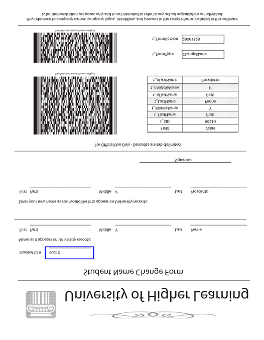
Let’s start with a flip augmentation:

1aug = A.Compose([
2    A.Flip(always_apply=True)
3], bbox_params=bbox_params)

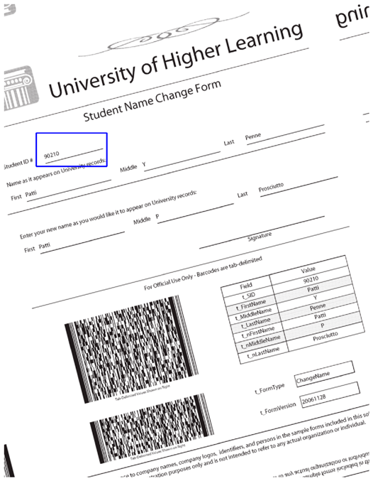
and rotate:

1aug = A.Compose([
2  A.Rotate(limit=80, always_apply=True)
3], bbox_params=bbox_params)

Another common difference between scanners can be simulated by changing the gamma of the images:

1aug = A.Compose([
2    A.RandomGamma(gamma_limit=(400, 500), always_apply=True)
3], bbox_params=bbox_params)

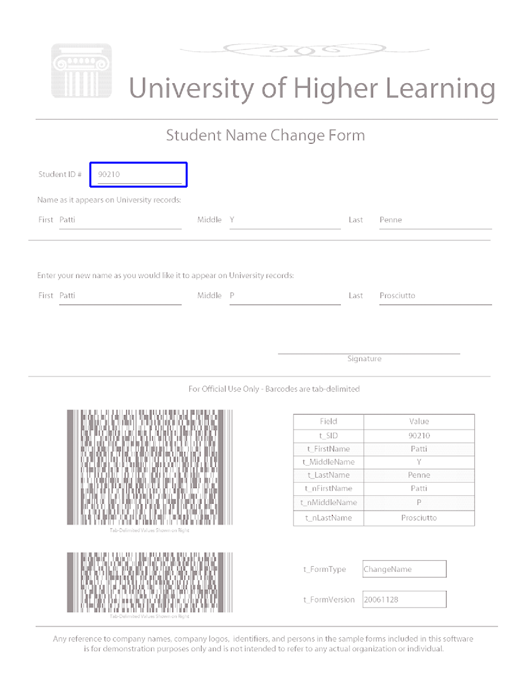
or adjusting the brightness and contrast:

1aug = A.Compose([
2    A.RandomBrightnessContrast(always_apply=True),
3], bbox_params=bbox_params)

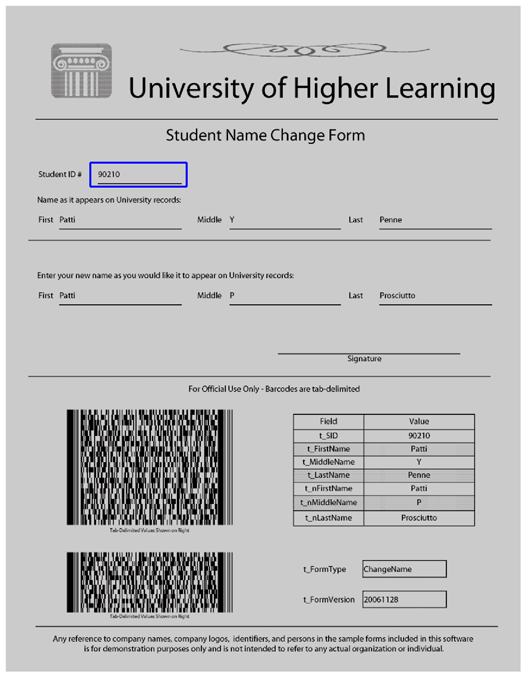
Incorrect color profiles can also be simulated with RGBShift:

1aug = A.Compose([
2    A.RGBShift(
3      always_apply=True,
4      r_shift_limit=100,
5      g_shift_limit=100,
6      b_shift_limit=100
7    ),
8], bbox_params=bbox_params)

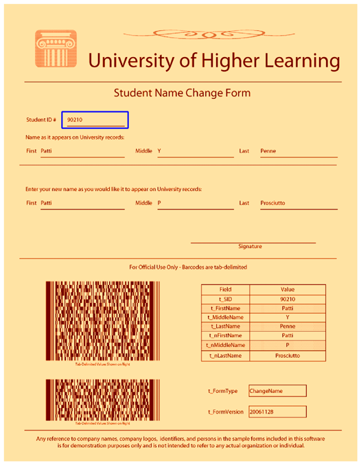
You can simulate hard to read documents by applying some noise:

1aug = A.Compose([
2    A.GaussNoise(
3      always_apply=True,
4      var_limit=(100, 300),
5      mean=150
6    ),
7], bbox_params=bbox_params)

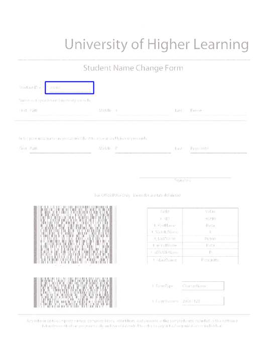
Creating Augmented Dataset

You’ve probably guessed that you can compose multiple augmentations. You can also choose how likely is to apply the specific transformation like so:

1doc_aug = A.Compose([
2    A.Flip(p=0.25),
3    A.RandomGamma(gamma_limit=(20, 300), p=0.5),
4    A.RandomBrightnessContrast(p=0.85),
5    A.Rotate(limit=35, p=0.9),
6    A.RandomRotate90(p=0.25),
7    A.RGBShift(p=0.75),
8    A.GaussNoise(p=0.25)
9], bbox_params=bbox_params)

You might want to quit with your image augmentation attempts right here. How can you correctly choose so many parameters? Furthermore, the parameters and augmentations might be highly domain-specific.

Luckily, the Albumentations Exploration Tool might help you explore different parameter configurations visually. You might even try to “learn” good augmentations. Learning Data Augmentation Strategies for Object Detection might be a first good read on the topic (source code included).

Object detection tasks have somewhat standard annotation format:

path/to/image.jpg, x1, y1, x2, y2, class_name

Let’s create 100 augmented images and save an annotation file for those:

1DATASET_PATH = 'data/augmented'
2IMAGES_PATH = f'{DATASET_PATH}/images'
3
4os.makedirs(DATASET_PATH, exist_ok=True)
5os.makedirs(IMAGES_PATH, exist_ok=True)
6
7rows = []
8for i in tqdm(range(100)):
9  augmented = doc_aug(
10    image=form,
11    bboxes=[STUDENT_ID_BBOX],
12    field_id=['1']
13  )
14  file_name = f'form_aug_{i}.jpg'
15  for bbox in augmented['bboxes']:
16    x_min, y_min, x_max, y_max = map(lambda v: int(v), bbox)
17    rows.append({
18      'file_name': f'images/{file_name}',
19      'x_min': x_min,
20      'y_min': y_min,
21      'x_max': x_max,
22      'y_max': y_max,
23      'class': 'student_id'
24    })
25
26  cv2.imwrite(f'{IMAGES_PATH}/{file_name}', augmented['image'])
27
28pd.DataFrame(rows).to_csv(
29  f'{DATASET_PATH}/annotations.csv',
30  header=True,
31  index=None
32)

Note that the code is somewhat generic and can handle multiple bounding boxes per image. You should easily be able to expand this code to handle multiple images from your dataset.

Conclusion

Great job! You can now add more training data for your models by augmenting images. We just scratched the surface of the Albumentation library. Feel free to explore and build even more powerful image augmentation pipelines!

You now know how to:

• Load images using OpenCV
• Apply various image augmentations
• Compose complex augmentations to simulate real-world data
• Create augmented dataset ready to use for Object Detection

Run the complete notebook in your browser

The complete project on GitHub

References

• Albumentations
• A survey on Image Data Augmentation for Deep Learning
• A Survey on Face Data Augmentation
• Learning Data Augmentation Strategies for Object Detection
• Albumentations Exploration Tool