Welcome to another part of the series. This time we will build a model that predicts the next word (a character actually) based on a few of the previous. We will extend it a bit by asking it for 5 suggestions instead of only 1. Similar models are widely used today. You might be using one without even knowing! Here’s one example:

Recurrent Neural Networks

Our weapon of choice for this task will be Recurrent Neural Networks (RNNs). But why? What’s wrong with the type of networks we’ve used so far? Nothing! Yet, they lack something that proves to be quite useful in practice - memory!

In short, RNN models provide a way to not only examine the current input but the one that was provided one step back, as well. If we turn that around, we can say that the decision reached at time step $t - 1$ directly affects the future at step $t$.

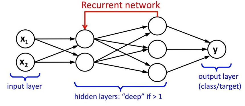
It seems like a waste to throw out the memory of what you’ve seen so far and start from scratch every time. That’s what other types of Neural Networks do. Let’s end this madness!

Definition

RNNs define a recurrence relation over time steps which is given by:

Where $S_t$ is the state at time step $t$, $X_t$ an exogenous input at time $t$, $W_{rec}$ and $W_x$ are weights parameters. The feedback loops gives memory to the model because it can remember information between time steps.

RNNs can compute the current state $S_t$ from the current input $X_t$ and previous state $S_{t-1}$ or predict the next state from $S_{t + 1}$ from the current $S_t$ and current input $X_t$. Concretely, we will pass a sequence of 40 characters and ask the model to predict the next one. We will append the new character and drop the first one and predict again. This will continue until we complete a whole word.

LSTMs

Two major problems torment the RNNs - vanishing and exploding gradients. In traditional RNNs the gradient signal can be multiplied a large number of times by the weight matrix. Thus, the magnitude of the weights of the transition matrix can play an important role.

If the weights in the matrix are small, the gradient signal becomes smaller at every training step, thus making learning very slow or completely stops it. This is called vanishing gradient. Let’s have a look at applying the sigmoid function multiple times, thus simulating the effect of vanishing gradient:

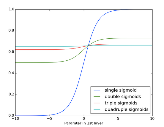
Conversely, the exploding gradient refers to the weights in this matrix being so large that it can cause learning to diverge.

LSTM model is a special kind of RNN that learns long-term dependencies. It introduces new structure - the memory cell that is composed of four elements: input, forget and output gates and a neuron that connects to itself:

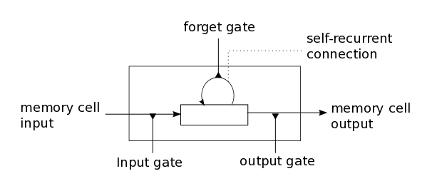
LSTMs fight the gradient vanishing problem by preserving the error that can be backpropagated through time and layers. By maintaining a more constant error, they allow for learning long-term dependencies. On another hand, exploding is controlled with gradient clipping, that is the gradient is not allowed to go above some predefined value.

Setup

Let’s properly seed our random number generator and import all required modules:

1import numpy as np
2np.random.seed(42)
3import tensorflow as tf
4tf.set_random_seed(42)
5from keras.models import Sequential, load_model
6from keras.layers import Dense, Activation
7from keras.layers import LSTM, Dropout
8from keras.layers import TimeDistributed
9from keras.layers.core import Dense, Activation, Dropout, RepeatVector
10from keras.optimizers import RMSprop
11import matplotlib.pyplot as plt
12import pickle
13import sys
14import heapq
15import seaborn as sns
16from pylab import rcParams
17
18%matplotlib inline
19
20sns.set(style='whitegrid', palette='muted', font_scale=1.5)
21
22rcParams['figure.figsize'] = 12, 5

This code works with TensorFlow 1.1 and Keras 2.

Loading the data

We will use Friedrich Nietzsche’s Beyond Good and Evil as a training corpus for our model. The text is not that large and our model can be trained relatively fast using a modest GPU. Let’s use the lowercase version of it:

1path = 'nietzsche.txt'
2text = open(path).read().lower()
3print('corpus length:', len(text))

1corpus length: 600893

Preprocessing

Let’s find all unique chars in the corpus and create char to index and index to char maps:

1chars = sorted(list(set(text)))
2char_indices = dict((c, i) for i, c in enumerate(chars))
3indices_char = dict((i, c) for i, c in enumerate(chars))
4
5print(f'unique chars: {len(chars)}')

1unique chars: 57

Next, let’s cut the corpus into chunks of 40 characters, spacing the sequences by 3 characters. Additionally, we will store the next character (the one we need to predict) for every sequence:

1SEQUENCE_LENGTH = 40
2step = 3
3sentences = []
4next_chars = []
5for i in range(0, len(text) - SEQUENCE_LENGTH, step):
6    sentences.append(text[i: i + SEQUENCE_LENGTH])
7    next_chars.append(text[i + SEQUENCE_LENGTH])
8print(f'num training examples: {len(sentences)}')

1num training examples: 200285

It is time for generating our features and labels. We will use the previously generated sequences and characters that need to be predicted to create one-hot encoded vectors using the char_indices map:

1X = np.zeros((len(sentences), SEQUENCE_LENGTH, len(chars)), dtype=np.bool)
2y = np.zeros((len(sentences), len(chars)), dtype=np.bool)
3for i, sentence in enumerate(sentences):
4    for t, char in enumerate(sentence):
5        X[i, t, char_indices[char]] = 1
6    y[i, char_indices[next_chars[i]]] = 1

Let’s have a look at a single training sequence:

1sentences[100]

1've been unskilled and unseemly methods f'

The character that needs to be predicted for it is:

1next_chars[100]

1'o'

The encoded (one-hot) data looks like this:

1X[0][0]

1array([False, False, False, False, False, False, False, False, False,
2       False, False, False, False, False, False, False, False, False,
3       False, False, False, False, False, False, False, False, False,
4       False, False, False, False, False, False, False, False, False,
5       False, False, False, False, False, False,  True, False, False,
6       False, False, False, False, False, False, False, False, False,
7       False, False, False], dtype=bool)

1y[0]

1array([False, False, False, False, False, False, False, False, False,
2       False, False, False, False, False, False, False, False, False,
3       False, False, False, False, False, False, False, False, False,
4       False, False, False, False, False, False, False, False, False,
5       False, False, False, False,  True, False, False, False, False,
6       False, False, False, False, False, False, False, False, False,
7       False, False, False], dtype=bool)

And for the dimensions:

1X.shape

1(200285, 40, 57)

1y.shape

1(200285, 57)

We have 200285 training examples, each sequence has length of 40 with 57 unique chars.

Building the model

The model we’re going to train is pretty straight forward. Single LSTM layer with 128 neurons which accepts input of shape (40 - the length of a sequence, 57 - the number of unique characters in our dataset). A fully connected layer (for our output) is added after that. It has 57 neurons and softmax for activation function:

1model = Sequential()
2model.add(LSTM(128, input_shape=(SEQUENCE_LENGTH, len(chars))))
3model.add(Dense(len(chars)))
4model.add(Activation('softmax'))

Training

Our model is trained for 20 epochs using RMSProp optimizer and uses 5% of the data for validation:

1optimizer = RMSprop(lr=0.01)
2model.compile(loss='categorical_crossentropy', optimizer=optimizer, metrics=['accuracy'])
3
4history = model.fit(X, y, validation_split=0.05, batch_size=128, epochs=20, shuffle=True).history

Saving

It took a lot of time to train our model. Let’s save our progress:

1model.save('keras_model.h5')
2pickle.dump(history, open("history.p", "wb"))

And load it back, just to make sure it works:

1model = load_model('keras_model.h5')
2history = pickle.load(open("history.p", "rb"))

Evaluation

Let’s have a look at how our accuracy and loss change over training epochs:

1plt.plot(history['acc'])
2plt.plot(history['val_acc'])
3plt.title('model accuracy')
4plt.ylabel('accuracy')
5plt.xlabel('epoch')
6plt.legend(['train', 'test'], loc='upper left');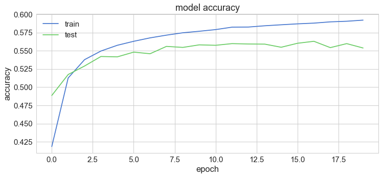

1plt.plot(history['loss'])
2plt.plot(history['val_loss'])
3plt.title('model loss')
4plt.ylabel('loss')
5plt.xlabel('epoch')
6plt.legend(['train', 'test'], loc='upper left');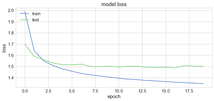

Let’s put our model to the test

Finally, it is time to predict some word completions using our model! First, we need some helper functions. Let’s start by preparing our input text:

1def prepare_input(text):
2    x = np.zeros((1, SEQUENCE_LENGTH, len(chars)))
3
4    for t, char in enumerate(text):
5        x[0, t, char_indices[char]] = 1.
6
7    return x

Remember that our sequences must be 40 characters long. So we make a tensor with shape (1, 40, 57), initialized with zeros. Then, a value of 1 is placed for each character in the passed text. We must not forget to use the lowercase version of the text:

1prepare_input("This is an example of input for our LSTM".lower())

1array([[[ 0.,  0.,  0., ...,  0.,  0.,  0.],
2        [ 0.,  0.,  0., ...,  0.,  0.,  0.],
3        [ 0.,  0.,  0., ...,  0.,  0.,  0.],
4        ...,
5        [ 0.,  0.,  0., ...,  0.,  0.,  0.],
6        [ 0.,  0.,  0., ...,  0.,  0.,  0.],
7        [ 0.,  0.,  0., ...,  0.,  0.,  0.]]])

Next up, the sample function:

1def sample(preds, top_n=3):
2    preds = np.asarray(preds).astype('float64')
3    preds = np.log(preds)
4    exp_preds = np.exp(preds)
5    preds = exp_preds / np.sum(exp_preds)
6
7    return heapq.nlargest(top_n, range(len(preds)), preds.take)

This function allows us to ask our model what are the next n most probable characters. Isn’t that heap just cool?

Now for the prediction functions themselves:

1def predict_completion(text):
2    original_text = text
3    generated = text
4    completion = ''
5    while True:
6        x = prepare_input(text)
7        preds = model.predict(x, verbose=0)[0]
8        next_index = sample(preds, top_n=1)[0]
9        next_char = indices_char[next_index]
10
11        text = text[1:] + next_char
12        completion += next_char
13
14        if len(original_text + completion) + 2 > len(original_text) and next_char == ' ':
15            return completion

This function predicts next character until space is predicted (you can extend that to punctuation symbols, right?). It does so by repeatedly preparing input, asking our model for predictions and sampling from them.

The final piece of the puzzle - predict_completions wraps everything and allow us to predict multiple completions:

1def predict_completions(text, n=3):
2    x = prepare_input(text)
3    preds = model.predict(x, verbose=0)[0]
4    next_indices = sample(preds, n)
5    return [indices_char[idx] + predict_completion(text[1:] + indices_char[idx]) for idx in next_indices]

Let’s use sequences of 40 characters that we will use as seed for our completions. All of these are quotes from Friedrich Nietzsche himself:

1quotes = [
2    "It is not a lack of love, but a lack of friendship that makes unhappy marriages.",
3    "That which does not kill us makes us stronger.",
4    "I'm not upset that you lied to me, I'm upset that from now on I can't believe you.",
5    "And those who were seen dancing were thought to be insane by those who could not hear the music.",
6    "It is hard enough to remember my opinions, without also remembering my reasons for them!"
7]

1for q in quotes:
2    seq = q[:40].lower()
3    print(seq)
4    print(predict_completions(seq, 5))
5    print()

1it is not a lack of love, but a lack of
2['the ', 'an ', 'such ', 'man ', 'present, ']
3
4that which does not kill us makes us str
5['ength ', 'uggle ', 'ong ', 'ange ', 'ive ']
6
7i'm not upset that you lied to me, i'm u
8['nder ', 'pon ', 'ses ', 't ', 'uder ']
9
10and those who were seen dancing were tho
11['se ', 're ', 'ugh ', ' servated ', 't ']
12
13it is hard enough to remember my opinion
14[' of ', 's ', ', ', '\nof ', 'ed ']

Apart from the fact that the completions look like proper words (remember, we are training our model on characters, not words), they look pretty reasonable as well! Perhaps better model and/or more training will provide even better results?

Conclusion

We’ve built a model using just a few lines of code in Keras that performs reasonably well after just 20 training epochs. Can you try it with your own text? Why not predict whole sentences? Will it work that well in other languages?

References

• Recurrent Nets in TensorFlow
• The Unreasonable Effectiveness of Recurrent Neural Networks
• Understanding LSTM Networks
• How to implement RNN in Python
• LSTM Networks for Sentiment Analysis
• cs231n - Recurrent Neural Networks