Curiousily

Making Twitter Cool Again

17.10.2016 — R, LDA, Text analysis — 3 min read

Have you spent some time on Twitter lately? So strange that politics is the main topic in so many tweets these days… Can we do something about it? YES!

I follow 124 tweeps at the time of this writing. You can see a list of them here. 200 of the most recent tweets for each account have been collected using the Twitter API. Here is what each row of our dataset contains:

text - text of the tweet
favorite_count
retweet_count
created_at - when the tweet was published
lang - language in which the tweet is written
user - screen name (username) of the user
user_tweet_count
user_following_count
user_followers_count
user_location

Only the text will be useful for us here. Feel free to use the other fields as well!

Loading libraries

Make sure you have installed and loaded the following libraries:

1library(tm)
2library(dplyr)
3library(doMC)
4library(RColorBrewer)
5library(wordcloud)
6library(ggplot2)
7library(SnowballC)
8library(topicmodels)
9library(LDAvis)

Let’s setup R and make our results reproducible.

1seed <- 42
2set.seed(seed)
3theme_set(theme_minimal())
4registerDoMC(cores = 4)
5options(warn=-1)

Load the data

1df <- read.csv("data/tweets.csv", header = T, stringsAsFactors = F)

Since our dataset is pretty well sorted (by username) we would love to randomize it a bit and tell R that created_at is an actual date field:

1df <- df[sample(nrow(df)),]
2rownames(df) <- 1:nrow(df)

1df$created_at <- as.Date(df$created_at)

1dim(df)

19948 x 10

We have a total of 19948 tweets - no missing data

Splitting the tweets

Let’s remove all non-ASCII characters and reserve only 10 tweets for testing:

1tweets <- iconv(df$text, to = "ASCII", sub = " ")
2train_tweets <- tweets[1:(nrow(df) - 10)]
3test_tweets <- tweets[(nrow(df) - 9):nrow(df)]

Preprocessing

Now, let’s prepare our text. Remove punctuations, numbers, URLs, stop words and apply stemming to the result.

1create_corpus <- function(data) {
2    data <- tolower(data)
3    data <- gsub("rt", " ", data)  # Remove retweets
4    data <- gsub("@\\w+", " ", data)  # Remove usernames
5    data <- gsub("http.+ |http.+$", " ", data)  # Remove links
6    data <- gsub("[[:punct:]]", " ", data)  # Remove punctuation
7    data <- gsub("[ |\t]{2,}", " ", data)  # Remove tabs
8    data <- gsub("amp", " ", data)  # Remove "&amp"
9    data <- gsub("^ ", "", data)  # Leading blanks
10    data <- gsub(" $", "", data)  # Lagging blanks
11    data <- gsub(" +", " ", data) # General white spaces
12    data <- unique(data)
13    VCorpus(VectorSource(data))
14}

1train_corpus <- create_corpus(train_tweets)

Our newly created corpus will be fed to a Document-Term matrix.

1dtm_train <- DocumentTermMatrix(train_corpus, control = list(
2    stemming = TRUE, removeNumbers = TRUE,
3    removePunctuation = TRUE,
4    stopwords = c(stopwords("en"), stopwords("SMART")),
5    wordLengths = c(3, 15)))
6dtm_train <- dtm_train[, !grepl("http", dtm_train$dimnames$Terms)]

Remove zero row entries

1row_totals <- apply(dtm_train , 1, sum)
2dtm_train <- dtm_train[row_totals > 0, ]

Exploration

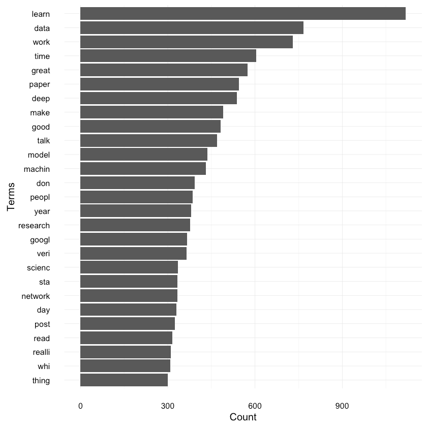
Let’s see which words are most used using our newly created corpus (set of documents).

1tdm_train <- TermDocumentMatrix(train_corpus, control = list(
2    stemming = TRUE, removeNumbers = TRUE,
3    removePunctuation = TRUE,
4    stopwords = c(stopwords("en"), stopwords("SMART")),
5    wordLengths = c(3, 15)))

1term_freq <- rowSums(as.matrix(tdm_train))
2term_freq <- subset(term_freq, term_freq >= 300)
3freq_df <- data.frame(term = names(term_freq), freq = term_freq)

1ggplot(freq_df, aes(x=reorder(term, freq), y=freq)) +
2    geom_bar(stat="identity") +
3    xlab("Terms") + ylab("Count") + coord_flip()

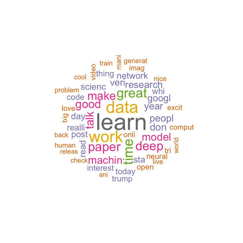
Want to make a guess what kind of tweeps I follow most? What about major topics?

Why not make a wordcloud using the same data?

1m <- as.matrix(tdm_train)
2word.freq <- sort(rowSums(m), decreasing = T)

1wordcloud(words = names(word.freq), freq = word.freq, min.freq = 200,
2random.order = F, colors=brewer.pal(8, "Dark2"))

We can even find associations in our corpus. Let’s see what is most associated to the word data?

1findAssocs(tdm_train, "data", 0.07)

word	strength
scienc	0.22
scientist	0.18
big	0.14
elixir	0.1
ingenu	0.1
janitor	0.1
servanda	0.1
mung	0.09
effici	0.08
literaci	0.08
driven	0.07

So it’s data science, data scientist, and big data? Looks reasonable enough!

Training our model

We will use the package topicmodels to train Latent Dirichlet Allocation (LDA) model using our tweet corpus. One good explanation of what exactly LDA is can be found on Quora. Concretely (get it?), we will use Gibbs sampling to find 10 (randomly picked number) topics.

1burnin <- 4000
2iter <- 2000
3thin <- 500
4lda <- LDA(dtm_train, k = 10, method = "Gibbs",
5            control = list(
6                burnin = burnin, thin = thin,
7                iter = iter, seed = seed
8            ))

Now that we trained our model, which words best describe each topic?

1terms(lda, 10)

1	2	3	4	5	6	7	8	9	10
time	learn	read	data	work	make	paper	peopl	great	googl
year	deep	nice	research	veri	good	open	don	talk	human
day	machin	lot	scienc	interest	thing	code	trump	today	game
world	model	show	big	cool	mani	python	whi	live	team
app	network	write	comput	problem	idea	releas	ani	excit	alphago
everi	post	love	futur	high	sta	result	realli	video	play
anoth	neural	book	program	thought	chang	sourc	question	week	deepmind
life	imag	mayb	machinelearn	impo	probabl	review	onli	workshop	experi
email	generat	pretti	intellig	ant	yeah	tool	doe	give	person
man	train	feel	predict	find	doesn	final	twitter	present	brain

Predicting topics of new data

Using the test data might not seem trivial at first, but creating corpus from the test tweets is a good first step.

1test_corpus <- create_corpus(test_tweets)

Let’s create Document-Term matrix using the test corpus and use our training matrix terms as a dictionary.

1dtm_test <- DocumentTermMatrix(test_corpus, control = list(
2    stemming = TRUE, removeNumbers = TRUE,
3    removePunctuation = TRUE,
4    stopwords = c(stopwords("en"), stopwords("SMART")),
5    dictionary=Terms(dtm_train), wordLengths = c(3, 15)))
6
7dtm_test <- dtm_test[, !grepl("http", dtm_test$dimnames$Terms)]
8row_totals <- apply(dtm_test , 1, sum)
9dtm_test   <- dtm_test[row_totals> 0, ]

Finally, assign topic probabilities to each tweet in our test dataset.

1lda_posterior <- posterior(lda, dtm_test)

Ready to have a look at the actual tweets?

1for(i in seq_along(test_tweets)) {
2    cat(paste(paste(i, test_tweets[i], sep = ": "), "\n\n"))
3}

11: Here I am at my new job at @King_Games and guess who shows up for a meeting? Jack Parmer ceo at @plotlygraphs !! :D https://t.co/EtuVWZcFzO
2
32: RT @ocelma: We're interested in both, but I wanted to stress today the implications of #wtf in #recsys https://t.co/sRZ2Re8W4u
4
53: RT @JordiTorresBCN:   Google ofrece m  s #MachineLearning a los desarrolladores!  https://t.co/yaLxQuL0BF #CloudComputing #TensorFlow https:/
6
74: Today's freshwater invert puzzling many... caddisflies! @freshwaterbio #namethatinvert https://t.co/EEZeTwnH0M
8
95: @dribnet impossible for Google to host the images themselves, because of legal issues. Large companies are a prime target for    lawsuits.
10
116: RT @polylogblog: Overheard at dinner re. decreasing importance of combinatorial algorithms: "these days, in order to sort, you first comput
12
137: RT @sedielem: Recurrent Spatial Transformer Networks by S  ren S  nderby et al. http://t.co/YJXyitvjko code: https://t.co/vYZcjbkmOH http://t
14
158: RT @skilpat: warren buffett had a 16% tax rate. praising him as some civic hero against trump is just as dumb as praising scrooge mcduck ov
16
179: RT @HeerJeet: 1. Let's step back and ask: what the fuck was Trump thinking when he ran for President?
18
1910: @usethespacebar @SpectralFilter @BecomingDataSci please also don't hesitate to ask any questions on github or the Jupyter mailing list!

Again, the top 5 terms for each topic:

1terms(lda, 5)

1	2	3	4	5	6	7	8	9	10
time	learn	read	data	work	make	paper	peopl	great	googl
year	deep	nice	research	veri	good	open	don	talk	human
day	machin	lot	scienc	interest	thing	code	trump	today	game
world	model	show	big	cool	mani	python	whi	live	team
app	network	write	comput	problem	idea	releas	ani	excit	alphago

What do you think about the results? Remember that every tweet is limited to 140 characters, thus our documents are rather small (even tiny considering preprocessing).

Let’s visualize our LDA model using the sweet LDAvis package.

1topicmodels2LDAvis <- function(x, ...){
2    post <- topicmodels::posterior(x)
3    mat <- x@wordassignments
4    LDAvis::createJSON(
5        phi = post[["terms"]],
6        theta = post[["topics"]],
7        vocab = colnames(post[["terms"]]),
8        doc.length = slam::row_sums(mat, na.rm = TRUE),
9        term.frequency = slam::col_sums(mat, na.rm = TRUE)
10    )
11}

1json <- lda %>% topicmodels2LDAvis()
2
3LDAvis::serVis(json, out.dir = 'twitter_lda_vis', open.browser = FALSE)

Take a look at the resulting visualization.

It looks like 3 (2, 4, 8) of the topics are pretty well separated from any other topic. We have 5 topics that are pretty close to each other on the bottom right. Might it be a good idea to try a different number of topics then?

At the end of the day, our model looks pretty useful. Let’s not forget that the data is pretty fresh and real (yes - I do not follow many tweeps, mostly those that are interested in math, machine learning and biotech/bioinformatics).

One could easily imagine using the trained model for making personalized recommendations of tweets based on preselected topics. Why not recommending new tweeps, too?

The LDA is very general and can be applied to any set of documents. Why not try it on papers, news or Facebook posts?

P. S. This post was written as an ipython notebook. Download it from here. The dataset can be download from here.

References

Want to be a Machine Learning expert?

Join the weekly newsletter on Data Science, Deep Learning and Machine Learning in your inbox, curated by me! Chosen by 10,000+ Machine Learning practitioners. (There might be some exclusive content, too!)

You'll never get spam from me

Hacker's Guide to Neural Networks in JavaScript

Build Machine Learning models (especially Deep Neural Networks) that you can easily integrate with existing or new web apps. Think of your ReactJs, Vue, or Angular app enhanced with the power of Machine Learning models.

Get SH*T Done with PyTorch

Learn how to solve real-world problems with Deep Learning models (NLP, Computer Vision, and Time Series). Go from prototyping to deployment with PyTorch and Python!

Hacker's Guide to Machine Learning with Python

This book brings the fundamentals of Machine Learning to you, using tools and techniques used to solve real-world problems in Computer Vision, Natural Language Processing, and Time Series analysis. The skills taught in this book will lay the foundation for you to advance your journey to Machine Learning Mastery!

Hands-On Machine Learning from Scratch

This book will guide you on your journey to deeper Machine Learning understanding by developing algorithms in Python from scratch! Learn why and when Machine learning is the right tool for the job and how to improve low performing models!