Curiousily

Multi-label Text Classification with BERT and PyTorch Lightning

26.04.2021 — Deep Learning, NLP, Neural Network, PyTorch, Python — 5 min read

TL;DR Learn how to prepare a dataset with toxic comments for multi-label text classification (tagging). We’ll fine-tune BERT using PyTorch Lightning and evaluate the model.

Multi-label text classification (or tagging text) is one of the most common tasks you’ll encounter when doing NLP. Modern Transformer-based models (like BERT) make use of pre-training on vast amounts of text data that makes fine-tuning faster, use fewer resources and more accurate on small(er) datasets.

In this tutorial, you’ll learn how to:

Load, balance and split text data into sets
Tokenize text (with BERT tokenizer) and create PyTorch dataset
Fine-tune BERT model with PyTorch Lightning
Find out about warmup steps and use a learning rate scheduler
Use area under the ROC and binary cross-entropy to evaluate the model during training
How to make predictions using the fine-tuned BERT model
Evaluate the performance of the model for each class (possible comment tag)

Will our model be any good for toxic text detection?

1import pandas as pd
2import numpy as np
3
4from tqdm.auto import tqdm
5
6import torch
7import torch.nn as nn
8from torch.utils.data import Dataset, DataLoader
9
10from transformers import BertTokenizerFast as BertTokenizer, BertModel, AdamW, get_linear_schedule_with_warmup
11
12import pytorch_lightning as pl
13from pytorch_lightning.metrics.functional import accuracy, f1, auroc
14from pytorch_lightning.callbacks import ModelCheckpoint, EarlyStopping
15from pytorch_lightning.loggers import TensorBoardLogger
16
17from sklearn.model_selection import train_test_split
18from sklearn.metrics import classification_report, multilabel_confusion_matrix
19
20import seaborn as sns
21from pylab import rcParams
22import matplotlib.pyplot as plt
23from matplotlib import rc
24
25%matplotlib inline
26%config InlineBackend.figure_format='retina'
27
28RANDOM_SEED = 42
29
30sns.set(style='whitegrid', palette='muted', font_scale=1.2)
31HAPPY_COLORS_PALETTE = ["#01BEFE", "#FFDD00", "#FF7D00", "#FF006D", "#ADFF02", "#8F00FF"]
32sns.set_palette(sns.color_palette(HAPPY_COLORS_PALETTE))
33rcParams['figure.figsize'] = 12, 8
34
35pl.seed_everything(RANDOM_SEED)

Data

Our dataset contains potentially offensive (toxic) comments and comes from the Toxic Comment Classification Challenge. Let’s start by download the data (from Google Drive):

1!gdown --id 1VuQ-U7TtggShMeuRSA_hzC8qGDl2LRkr

Let’s load and look at the data:

1df = pd.read_csv("toxic_comments.csv")
2df.head()

	id	comment_text
0	0000997932d777bf	Explanation\nWhy the edits made under my usern...
1	000103f0d9cfb60f	D'aww! He matches this background colour I'm s...
2	000113f07ec002fd	Hey man, I'm really not trying to edit war. It...
3	0001b41b1c6bb37e	"\nMore\nI can't make any real suggestions on ...
4	0001d958c54c6e35	You, sir, are my hero. Any chance you remember...

We have text (comment) and six different toxic labels. Note that we have clean content, too.

Let’s split the data:

1train_df, val_df = train_test_split(df, test_size=0.05)
2train_df.shape, val_df.shape

1((151592, 8), (7979, 8))

Preprocessing

Let’s look at the distribution of the labels:

1LABEL_COLUMNS = df.columns.tolist()[2:]
2df[LABEL_COLUMNS].sum().sort_values().plot(kind="barh");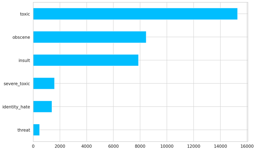

We have a severe case of imbalance. But that is not the full picture. What about the toxic vs clean comments?

1train_toxic = train_df[train_df[LABEL_COLUMNS].sum(axis=1) > 0]
2train_clean = train_df[train_df[LABEL_COLUMNS].sum(axis=1) == 0]
3
4pd.DataFrame(dict(
5  toxic=[len(train_toxic)],
6  clean=[len(train_clean)]
7)).plot(kind='barh');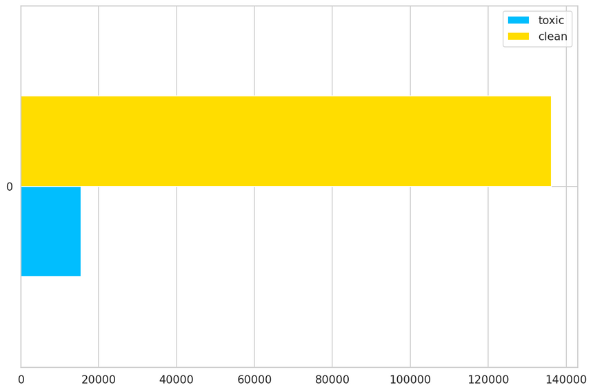

Clean vs toxic comment count in the dataset

Again, we have a severe imbalance in favor of the clean comments. To combat this, we’ll sample 15,000 examples from the clean comments and create a new training set:

1train_df = pd.concat([
2  train_toxic,
3  train_clean.sample(15_000)
4])
5
6train_df.shape, val_df.shape

1((30427, 8), (7979, 8))

Tokenization

We need to convert the raw text into a list of tokens. For that, we’ll use the built-in BertTokenizer:

1BERT_MODEL_NAME = 'bert-base-cased'
2tokenizer = BertTokenizer.from_pretrained(BERT_MODEL_NAME)

Let’s try it out on a sample comment:

1sample_row = df.iloc[16]
2sample_comment = sample_row.comment_text
3sample_labels = sample_row[LABEL_COLUMNS]
4
5print(sample_comment)
6print()
7print(sample_labels.to_dict())

1Bye!
2
3Don't look, come or think of comming back! Tosser.
4
5{'toxic': 1, 'severe_toxic': 0, 'obscene': 0, 'threat': 0, 'insult': 0, 'identity_hate': 0}

1encoding = tokenizer.encode_plus(
2  sample_comment,
3  add_special_tokens=True,
4  max_length=512,
5  return_token_type_ids=False,
6  padding="max_length",
7  return_attention_mask=True,
8  return_tensors='pt',
9)
10
11encoding.keys()

1dict_keys(['input_ids', 'attention_mask'])

1encoding["input_ids"].shape, encoding["attention_mask"].shape

1(torch.Size([1, 512]), torch.Size([1, 512]))

The result of the encoding is a dictionary with token ids input_ids and an attention mask attention_mask (which tokens should be used by the model 1 - use or 0 - don’t use).

Let’s look at their contents:

1encoding["input_ids"].squeeze()[:20]

1tensor([  101, 17774,   106,  1790,   112,   189,  1440,   117,  1435,  1137,
2             1341,  1104,  3254,  5031,  1171,   106,  1706, 14607,   119,   102])

1encoding["attention_mask"].squeeze()[:20]

1tensor([1, 1, 1, 1, 1, 1, 1, 1, 1, 1, 1, 1, 1, 1, 1, 1, 1, 1, 1, 1])

You can also inverse the tokenization and get back (kinda) the words from the token ids:

1print(tokenizer.convert_ids_to_tokens(encoding["input_ids"].squeeze())[:20])

1['[CLS]', 'Bye', '!', 'Don', "'", 't', 'look', ',', 'come', 'or', 'think', 'of', 'com', '##ming', 'back', '!', 'To', '##sser', '.', '[SEP]']

We need to specify the maximum number of tokens when encoding (512 is the maximum we can do). Let’s check the number of tokens per comment:

1token_counts = []
2
3for _, row in train_df.iterrows():
4  token_count = len(tokenizer.encode(
5    row["comment_text"],
6    max_length=512,
7    truncation=True
8  ))
9  token_counts.append(token_count)

1sns.histplot(token_counts)
2plt.xlim([0, 512]);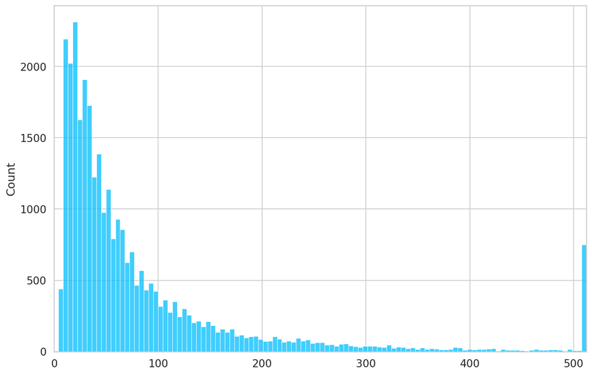

Most of the comments contain less than 300 tokens or more than 512. So, we’ll stick with the limit of 512.

1MAX_TOKEN_COUNT = 512

Dataset

We’ll wrap the tokenization process in a PyTorch Dataset, along with converting the labels to tensors:

1class ToxicCommentsDataset(Dataset):
2
3  def __init__(
4    self,
5    data: pd.DataFrame,
6    tokenizer: BertTokenizer,
7    max_token_len: int = 128
8  ):
9    self.tokenizer = tokenizer
10    self.data = data
11    self.max_token_len = max_token_len
12
13  def __len__(self):
14    return len(self.data)
15
16  def __getitem__(self, index: int):
17    data_row = self.data.iloc[index]
18
19    comment_text = data_row.comment_text
20    labels = data_row[LABEL_COLUMNS]
21
22    encoding = self.tokenizer.encode_plus(
23      comment_text,
24      add_special_tokens=True,
25      max_length=self.max_token_len,
26      return_token_type_ids=False,
27      padding="max_length",
28      truncation=True,
29      return_attention_mask=True,
30      return_tensors='pt',
31    )
32
33    return dict(
34      comment_text=comment_text,
35      input_ids=encoding["input_ids"].flatten(),
36      attention_mask=encoding["attention_mask"].flatten(),
37      labels=torch.FloatTensor(labels)
38    )

Let’s have a look at a sample item from the dataset:

1train_dataset = ToxicCommentsDataset(
2  train_df,
3  tokenizer,
4  max_token_len=MAX_TOKEN_COUNT
5)
6
7sample_item = train_dataset[0]
8sample_item.keys()

1dict_keys(['comment_text', 'input_ids', 'attention_mask', 'labels'])

1sample_item["comment_text"]

1'Hi, ya fucking idiot. ^_^'

1sample_item["labels"]

1tensor([1., 0., 1., 0., 1., 0.])

1sample_item["input_ids"].shape

1torch.Size([512])

Let’s load the BERT model and pass a sample of batch data through:

1bert_model = BertModel.from_pretrained(BERT_MODEL_NAME, return_dict=True)
2
3sample_batch = next(iter(DataLoader(train_dataset, batch_size=8, num_workers=2)))
4sample_batch["input_ids"].shape, sample_batch["attention_mask"].shape

1(torch.Size([8, 512]), torch.Size([8, 512]))

1output = bert_model(sample_batch["input_ids"], sample_batch["attention_mask"])

1output.last_hidden_state.shape, output.pooler_output.shape

1(torch.Size([8, 512, 768]), torch.Size([8, 768]))

The 768 dimension comes from the BERT hidden size:

1bert_model.config.hidden_size

The larger version of BERT has more attention heads and a larger hidden size.

We’ll wrap our custom dataset into a LightningDataModule:

1class ToxicCommentDataModule(pl.LightningDataModule):
2
3  def __init__(self, train_df, test_df, tokenizer, batch_size=8, max_token_len=128):
4    super().__init__()
5    self.batch_size = batch_size
6    self.train_df = train_df
7    self.test_df = test_df
8    self.tokenizer = tokenizer
9    self.max_token_len = max_token_len
10
11  def setup(self, stage=None):
12    self.train_dataset = ToxicCommentsDataset(
13      self.train_df,
14      self.tokenizer,
15      self.max_token_len
16    )
17
18    self.test_dataset = ToxicCommentsDataset(
19      self.test_df,
20      self.tokenizer,
21      self.max_token_len
22    )
23
24  def train_dataloader(self):
25    return DataLoader(
26      self.train_dataset,
27      batch_size=self.batch_size,
28      shuffle=True,
29      num_workers=2
30    )
31
32  def val_dataloader(self):
33    return DataLoader(
34      self.test_dataset,
35      batch_size=self.batch_size,
36      num_workers=2
37    )
38
39  def test_dataloader(self):
40    return DataLoader(
41      self.test_dataset,
42      batch_size=self.batch_size,
43      num_workers=2
44    )

ToxicCommentDataModule encapsulates all data loading logic and returns the necessary data loaders. Let’s create an instance of our data module:

1N_EPOCHS = 10
2BATCH_SIZE = 12
3
4data_module = ToxicCommentDataModule(
5  train_df,
6  val_df,
7  tokenizer,
8  batch_size=BATCH_SIZE,
9  max_token_len=MAX_TOKEN_COUNT
10)

Model

Our model will use a pre-trained BertModel and a linear layer to convert the BERT representation to a classification task. We’ll pack everything in a LightningModule:

1class ToxicCommentTagger(pl.LightningModule):
2
3  def __init__(self, n_classes: int, n_training_steps=None, n_warmup_steps=None):
4    super().__init__()
5    self.bert = BertModel.from_pretrained(BERT_MODEL_NAME, return_dict=True)
6    self.classifier = nn.Linear(self.bert.config.hidden_size, n_classes)
7    self.n_training_steps = n_training_steps
8    self.n_warmup_steps = n_warmup_steps
9    self.criterion = nn.BCELoss()
10
11  def forward(self, input_ids, attention_mask, labels=None):
12    output = self.bert(input_ids, attention_mask=attention_mask)
13    output = self.classifier(output.pooler_output)
14    output = torch.sigmoid(output)
15    loss = 0
16    if labels is not None:
17        loss = self.criterion(output, labels)
18    return loss, output
19
20  def training_step(self, batch, batch_idx):
21    input_ids = batch["input_ids"]
22    attention_mask = batch["attention_mask"]
23    labels = batch["labels"]
24    loss, outputs = self(input_ids, attention_mask, labels)
25    self.log("train_loss", loss, prog_bar=True, logger=True)
26    return {"loss": loss, "predictions": outputs, "labels": labels}
27
28  def validation_step(self, batch, batch_idx):
29    input_ids = batch["input_ids"]
30    attention_mask = batch["attention_mask"]
31    labels = batch["labels"]
32    loss, outputs = self(input_ids, attention_mask, labels)
33    self.log("val_loss", loss, prog_bar=True, logger=True)
34    return loss
35
36  def test_step(self, batch, batch_idx):
37    input_ids = batch["input_ids"]
38    attention_mask = batch["attention_mask"]
39    labels = batch["labels"]
40    loss, outputs = self(input_ids, attention_mask, labels)
41    self.log("test_loss", loss, prog_bar=True, logger=True)
42    return loss
43
44  def training_epoch_end(self, outputs):
45
46    labels = []
47    predictions = []
48    for output in outputs:
49      for out_labels in output["labels"].detach().cpu():
50        labels.append(out_labels)
51      for out_predictions in output["predictions"].detach().cpu():
52        predictions.append(out_predictions)
53
54    labels = torch.stack(labels).int()
55    predictions = torch.stack(predictions)
56
57    for i, name in enumerate(LABEL_COLUMNS):
58      class_roc_auc = auroc(predictions[:, i], labels[:, i])
59      self.logger.experiment.add_scalar(f"{name}_roc_auc/Train", class_roc_auc, self.current_epoch)
60
61
62  def configure_optimizers(self):
63
64    optimizer = AdamW(self.parameters(), lr=2e-5)
65
66    scheduler = get_linear_schedule_with_warmup(
67      optimizer,
68      num_warmup_steps=self.n_warmup_steps,
69      num_training_steps=self.n_training_steps
70    )
71
72    return dict(
73      optimizer=optimizer,
74      lr_scheduler=dict(
75        scheduler=scheduler,
76        interval='step'
77      )
78    )

Most of the implementation is just a boilerplate. Two points of interest are the way we configure the optimizers and calculating the area under ROC. We’ll dive a bit deeper into those next.

Optimizer scheduler

The job of a scheduler is to change the learning rate of the optimizer during training. This might lead to better performance of our model. We’ll use the get_linear_schedule_with_warmup.

Let’s have a look at a simple example to make things clearer:

1dummy_model = nn.Linear(2, 1)
2
3optimizer = AdamW(params=dummy_model.parameters(), lr=0.001)
4
5warmup_steps = 20
6total_training_steps = 100
7
8scheduler = get_linear_schedule_with_warmup(
9  optimizer,
10  num_warmup_steps=warmup_steps,
11  num_training_steps=total_training_steps
12)
13
14learning_rate_history = []
15
16for step in range(total_training_steps):
17  optimizer.step()
18  scheduler.step()
19  learning_rate_history.append(optimizer.param_groups[0]['lr'])

1plt.plot(learning_rate_history, label="learning rate")
2plt.axvline(x=warmup_steps, color="red", linestyle=(0, (5, 10)), label="warmup end")
3plt.legend()
4plt.xlabel("Step")
5plt.ylabel("Learning rate")
6plt.tight_layout();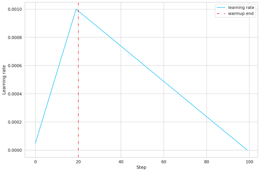

Linear learning rate scheduling over training steps

We simulate 100 training steps and tell the scheduler to warm up for the first 20. The learning rate grows to the initial fixed value of 0.001 during the warm-up and then goes down (linearly) to 0.

To use the scheduler, we need to calculate the number of training and warm-up steps. The number of training steps per epoch is equal to number of training examples / batch size. The number of total training steps is training steps per epoch * number of epochs:

1steps_per_epoch=len(train_df) // BATCH_SIZE
2total_training_steps = steps_per_epoch * N_EPOCHS

We’ll use a fifth of the training steps for a warm-up:

1warmup_steps = total_training_steps // 5
2warmup_steps, total_training_steps

1(5070, 25350)

We can now create an instance of our model:

1model = ToxicCommentTagger(
2  n_classes=len(LABEL_COLUMNS),
3  n_warmup_steps=warmup_steps,
4  n_training_steps=total_training_steps
5)

Evaluation

Multi-label classification boils down to doing binary classification for each label/tag.

We’ll use Binary Cross Entropy to measure the error for each label. PyTorch has BCELoss, which we’re going to combine with a sigmoid function (as we did in the model implementation). Let’s look at an example:

1criterion = nn.BCELoss()
2
3prediction = torch.FloatTensor(
4  [10.95873564, 1.07321467, 1.58524066, 0.03839076, 15.72987556, 1.09513213]
5)
6labels = torch.FloatTensor(
7  [1., 0., 0., 0., 1., 0.]
8)

1torch.sigmoid(prediction)

1tensor([1.0000, 0.7452, 0.8299, 0.5096, 1.0000, 0.7493])

1criterion(torch.sigmoid(prediction), labels)

1tensor(0.8725)

We can use the same approach to calculate the loss of the predictions:

1_, predictions = model(sample_batch["input_ids"], sample_batch["attention_mask"])
2predictions

1tensor([[0.3963, 0.6318, 0.6543, 0.5179, 0.4099, 0.4998],
2            [0.4008, 0.6165, 0.6733, 0.5460, 0.4378, 0.5083],
3            [0.3877, 0.6185, 0.6830, 0.5238, 0.4326, 0.5138],
4            [0.3910, 0.6206, 0.6658, 0.5431, 0.4396, 0.5002],
5            [0.3792, 0.6241, 0.6508, 0.5347, 0.4374, 0.5110],
6            [0.4069, 0.6106, 0.7019, 0.5484, 0.4450, 0.4995],
7            [0.3861, 0.6135, 0.6867, 0.5179, 0.4525, 0.5188],
8            [0.3819, 0.6081, 0.6821, 0.5227, 0.4419, 0.5246]],
9           grad_fn=<SigmoidBackward>)

1criterion(predictions, sample_batch["labels"])

1tensor(0.8056, grad_fn=<BinaryCrossEntropyBackward>)

ROC Curve

Another metric we’re going to use is the area under the Receiver operating characteristic (ROC) for each tag. ROC is created by plotting the True Positive Rate (TPR) vs False Positive Rate (FPR):

\text{TPR} = \frac{\text{TP}}{\text{TP} \text{+} \text{FN}}

\text{FPR} = \frac{\text{FP}}{\text{FP} \text{+} \text{TN}}

1from sklearn import metrics
2
3fpr = [0.        , 0.        , 0.        , 0.02857143, 0.02857143,
4       0.11428571, 0.11428571, 0.2       , 0.4       , 1.        ]
5
6tpr = [0.        , 0.01265823, 0.67202532, 0.76202532, 0.91468354,
7       0.97468354, 0.98734177, 0.98734177, 1.        , 1.        ]
8
9_, ax = plt.subplots()
10ax.plot(fpr, tpr, label="ROC")
11ax.plot([0.05, 0.95], [0.05, 0.95], transform=ax.transAxes, label="Random classifier", color="red")
12ax.legend(loc=4)
13ax.set_xlabel("False positive rate")
14ax.set_ylabel("True positive rate")
15ax.set_title("Example ROC curve")
16plt.show();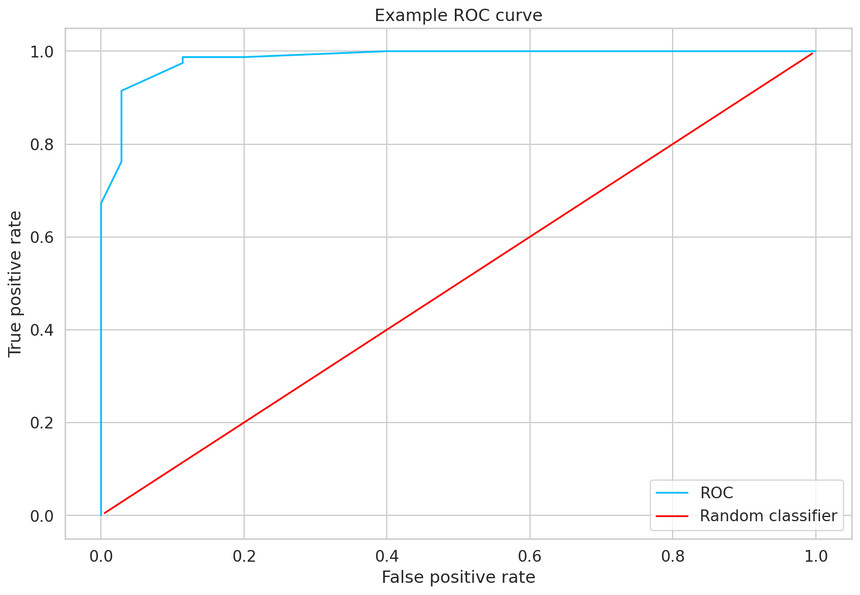

Example ROC vaue of a trained classifier vs random classifier

Training

The beauty of PyTorch Lightning is that you can build a standard pipeline that you like and train (almost?) every model you might imagine. I prefer to use at least 3 components.

Checkpointing that saves the best model (based on validation loss):

1checkpoint_callback = ModelCheckpoint(
2  dirpath="checkpoints",
3  filename="best-checkpoint",
4  save_top_k=1,
5  verbose=True,
6  monitor="val_loss",
7  mode="min"
8)

Log the progress in TensorBoard:

1logger = TensorBoardLogger("lightning_logs", name="toxic-comments")

And early stopping triggers when the loss hasn’t improved for the last 2 epochs (you might want to remove/reconsider this when training on real-world projects):

1early_stopping_callback = EarlyStopping(monitor='val_loss', patience=2)

We can start the training process:

1trainer = pl.Trainer(
2  logger=logger,
3  checkpoint_callback=checkpoint_callback,
4  callbacks=[early_stopping_callback],
5  max_epochs=N_EPOCHS,
6  gpus=1,
7  progress_bar_refresh_rate=30
8)

1GPU available: True, used: True
2TPU available: False, using: 0 TPU cores

1trainer.fit(model, data_module)

1LOCAL_RANK: 0 - CUDA_VISIBLE_DEVICES: [0]
2
3  | Name       | Type      | Params
4-----------------------------------------
50 | bert       | BertModel | 108 M
61 | classifier | Linear    | 4.6 K
72 | criterion  | BCELoss   | 0
8-----------------------------------------
9108 M     Trainable params
100         Non-trainable params
11108 M     Total params
12433.260   Total estimated model params size (MB)
13
14
15Epoch 0, global step 2535: val_loss reached 0.05723 (best 0.05723), saving model to "/content/checkpoints/best-checkpoint.ckpt" as top 1
16
17Epoch 1, global step 5071: val_loss reached 0.04705 (best 0.04705), saving model to "/content/checkpoints/best-checkpoint.ckpt" as top 1
18
19Epoch 2, step 7607: val_loss was not in top 1
20
21Epoch 3, step 10143: val_loss was not in top 1

The model improved for (only) 2 epochs. We’ll have to evaluate it to see whether it is any good. Let’s double-check the validation loss:

1trainer.test()

1LOCAL_RANK: 0 - CUDA_VISIBLE_DEVICES: [0]
2
3--------------------------------------------------------------------------------
4DATALOADER:0 TEST RESULTS
5{'test_loss': 0.04704693332314491}
6--------------------------------------------------------------------------------
7
8[{'test_loss': 0.04704693332314491}]

Predictions

I like to look at a small sample of predictions after the training is complete. This builds intuition about the quality of the predictions (qualitative evaluation).

Let’s load the best version (according to the validation loss) of our model:

1trained_model = ToxicCommentTagger.load_from_checkpoint(
2  trainer.checkpoint_callback.best_model_path,
3  n_classes=len(LABEL_COLUMNS)
4)
5trained_model.eval()
6trained_model.freeze()

We put our model into “eval” mode, and we’re ready to make some predictions. Here’s the prediction on a sample (totally fictional) comment:

1test_comment = "Hi, I'm Meredith and I'm an alch... good at supplier relations"
2
3encoding = tokenizer.encode_plus(
4  test_comment,
5  add_special_tokens=True,
6  max_length=512,
7  return_token_type_ids=False,
8  padding="max_length",
9  return_attention_mask=True,
10  return_tensors='pt',
11)
12
13_, test_prediction = trained_model(encoding["input_ids"], encoding["attention_mask"])
14test_prediction = test_prediction.flatten().numpy()
15
16for label, prediction in zip(LABEL_COLUMNS, test_prediction):
17  print(f"{label}: {prediction}")

1toxic: 0.02174694836139679
2severe_toxic: 0.0013127995189279318
3obscene: 0.0035953170154243708
4threat: 0.0015959267038851976
5insult: 0.003400973277166486
6identity_hate: 0.003609051927924156

Looks good. This one is pretty clean. We’ll reduce the noise of the predictions by thresholding (0.5) them. We’ll take only tag predictions above (or equal) to the threshold. Let’s try something toxic:

1THRESHOLD = 0.5
2
3test_comment = "You are such a loser! You'll regret everything you've done to me!"
4encoding = tokenizer.encode_plus(
5  test_comment,
6  add_special_tokens=True,
7  max_length=512,
8  return_token_type_ids=False,
9  padding="max_length",
10  return_attention_mask=True,
11  return_tensors='pt',
12)
13
14_, test_prediction = trained_model(encoding["input_ids"], encoding["attention_mask"])
15test_prediction = test_prediction.flatten().numpy()
16
17for label, prediction in zip(LABEL_COLUMNS, test_prediction):
18  if prediction < THRESHOLD:
19    continue
20  print(f"{label}: {prediction}")

1toxic: 0.9569520354270935
2insult: 0.7289626002311707

I definitely agree with those tags. It looks like our model is doing something reasonable, on those two examples.

Evaluation

Let’s get a more complete overview of the performance of our model. We’ll start by taking all predictions and labels from the validation set:

1device = torch.device('cuda' if torch.cuda.is_available() else 'cpu')
2trained_model = trained_model.to(device)
3
4val_dataset = ToxicCommentsDataset(
5  val_df,
6  tokenizer,
7  max_token_len=MAX_TOKEN_COUNT
8)
9
10predictions = []
11labels = []
12
13for item in tqdm(val_dataset):
14  _, prediction = trained_model(
15    item["input_ids"].unsqueeze(dim=0).to(device),
16    item["attention_mask"].unsqueeze(dim=0).to(device)
17  )
18  predictions.append(prediction.flatten())
19  labels.append(item["labels"].int())
20
21predictions = torch.stack(predictions).detach().cpu()
22labels = torch.stack(labels).detach().cpu()

One simple metric is the accuracy of the model:

1accuracy(predictions, labels, threshold=THRESHOLD)

1tensor(0.9813)

That’s great, but you should take this result with a grain of salt. We have a very imbalanced dataset. Let’s check the ROC for each tag:

1print("AUROC per tag")
2for i, name in enumerate(LABEL_COLUMNS):
3  tag_auroc = auroc(predictions[:, i], labels[:, i], pos_label=1)
4  print(f"{name}: {tag_auroc}")

1AUROC per tag
2  toxic: 0.985722541809082
3  severe_toxic: 0.990084171295166
4  obscene: 0.995059609413147
5  threat: 0.9909615516662598
6  insult: 0.9884428977966309
7  identity_hate: 0.9890572428703308

Very good results, but just before we go party, let’s check the classification report for each class. To make this work, we must apply thresholding to the predictions:

1y_pred = predictions.numpy()
2y_true = labels.numpy()
3
4upper, lower = 1, 0
5
6y_pred = np.where(y_pred > THRESHOLD, upper, lower)
7
8print(classification_report(
9  y_true,
10  y_pred,
11  target_names=LABEL_COLUMNS,
12  zero_division=0
13))

1precision    recall  f1-score   support
2
3            toxic       0.68      0.91      0.78       748
4     severe_toxic       0.53      0.30      0.38        80
5          obscene       0.79      0.87      0.83       421
6           threat       0.23      0.38      0.29        13
7           insult       0.79      0.70      0.74       410
8    identity_hate       0.59      0.62      0.60        71
9
10        micro avg       0.72      0.81      0.76      1743
11        macro avg       0.60      0.63      0.60      1743
12     weighted avg       0.72      0.81      0.75      1743
13      samples avg       0.08      0.08      0.08      1743

That gives us a much more realistic picture of the overall performance. The model makes mistakes on the tags will low amounts of examples. What can you do about it?

Summary

Great job, you have a model that can tell (to some extent) if a text is toxic (and what kind) or not! Fine-tuning modern pre-trained Transformer models allow you to get high accuracy on a variety of NLP tasks with little compute power and small datasets.

In this tutorial, you’ll learned how to:

Load, balance and split text data into sets
Tokenize text (with BERT tokenizer) and create PyTorch dataset
Fine-tune BERT model with PyTorch Lightning
Find out about warmup steps and use a learning rate scheduler
Use area under the ROC and binary cross-entropy to evaluate the model during training
How to make predictions using the fine-tuned BERT model
Evaluate the performance of the model for each class (possible comment tag)

Can you increase the accuracy of the model? How about better parameters or different learning rate scheduling? Let me know in the comments.

References

Want to be a Machine Learning expert?

Join the weekly newsletter on Data Science, Deep Learning and Machine Learning in your inbox, curated by me! Chosen by 10,000+ Machine Learning practitioners. (There might be some exclusive content, too!)

You'll never get spam from me

Hacker's Guide to Neural Networks in JavaScript

Build Machine Learning models (especially Deep Neural Networks) that you can easily integrate with existing or new web apps. Think of your ReactJs, Vue, or Angular app enhanced with the power of Machine Learning models.

Get SH*T Done with PyTorch

Learn how to solve real-world problems with Deep Learning models (NLP, Computer Vision, and Time Series). Go from prototyping to deployment with PyTorch and Python!

Hacker's Guide to Machine Learning with Python

This book brings the fundamentals of Machine Learning to you, using tools and techniques used to solve real-world problems in Computer Vision, Natural Language Processing, and Time Series analysis. The skills taught in this book will lay the foundation for you to advance your journey to Machine Learning Mastery!

Hands-On Machine Learning from Scratch

This book will guide you on your journey to deeper Machine Learning understanding by developing algorithms in Python from scratch! Learn why and when Machine learning is the right tool for the job and how to improve low performing models!