Music artist Recommender System using Stochastic Gradient Descent | Machine Learning from Scratch (Part VII)
— Machine Learning, Collaborative Filtering, Recommender Systems, Gradient Descent — 7 min read
Share
TL;DR Build a Recommender System in Python from scratch. Create ratings matrix from last.fm dataset and preprocess the data. Train the model using Stochastic Gradient Descent (SGD) and use it to recommend music artists.
Recommender Systems are becoming more and more relevant as the amount of information on “The Internets” is exponentially increasing:

Finding what you might enjoy from books, movies, games to who to follow on Instagram becomes increasingly difficult. Moreover, we (the users) require faster interactions with the products we use on a daily basis, so we don’t feel like we waste time (even though we do it more than ever before in human history). As the amounts of data increase, your computational resources might have a hard time to produce fast enough results.
Here, we’ll have a look at a succinct implementation of a Recommender System that is both the basis of many real-world implementations and is easy to understand. I can highly recommend you to read this through :)
Complete source code in Google Colaboratory Notebook
User Ratings
Traditionally, recommender systems are built around user ratings given for a set of items, e.g. movie ratings on IMDB. Here, we’ll have a look at using another metric for making recommendations.
Our data comes from last.fm, hosted by GroupLens (download from here). It contains the following:
- user_artists.dat - userID, artistID, weight - plays of artist by user.
- artists.dat - id, name, url, pictureURL
- tags.dat - tagID, tagValue
- user_taggedartists.dat - userID, artistID, tagID, day, month, year
- user_taggedartists-timestamps.dat - userID, artistID, tagID, timestamp
- user_friends.dat - userID, friendID. User/friend relationships.
We’ll focus on user_artists.dat and artists.dat as they contain all data required to make recommendations for new music artists to a user. Instead of ratings, we’re going to use the play count by a user for each artist.
Loading the data
Let’s load the data into Pandas data frames:
1plays = pd.read_csv('user_artists.dat', sep='\t')2artists = pd.read_csv(3 'artists.dat',4 sep='\t',5 usecols=['id','name']6)Data wrangling
You need to do a bit of wrangling before working with the data:
1ap = pd.merge(2 artists, plays,3 how="inner",4 left_on="id",5 right_on="artistID"6)7ap = ap.rename(columns={"weight": "playCount"})We merge the artists and user plays and rename the weight column to playCount. Let’s rank the artists based on how much they were played by the users:
1artist_rank = ap.groupby(['name']) \2 .agg({'userID' : 'count', 'playCount' : 'sum'}) \3 .rename(columns={"userID" : 'totalUniqueUsers', "playCount" : "totalArtistPlays"}) \4 .sort_values(['totalArtistPlays'], ascending=False)56artist_rank['avgUserPlays'] = artist_rank['totalArtistPlays'] / artist_rank['totalUniqueUsers']And merge the results with the previous data frame:
1ap = ap.join(artist_rank, on="name", how="inner") \2 .sort_values(['playCount'], ascending=False)Here is a subset of the data:
| name | userID | artistID | playCount |
|---|---|---|---|
| Depeche Mode | 1642 | 72 | 352698 |
| Thalía | 2071 | 792 | 324663 |
| U2 | 1094 | 511 | 320725 |
| Blur | 1905 | 203 | 257978 |
| Paramore | 1664 | 498 | 227829 |
Exploration
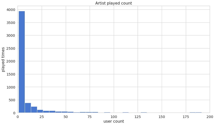
Let’s look at how much each artist is played by users:
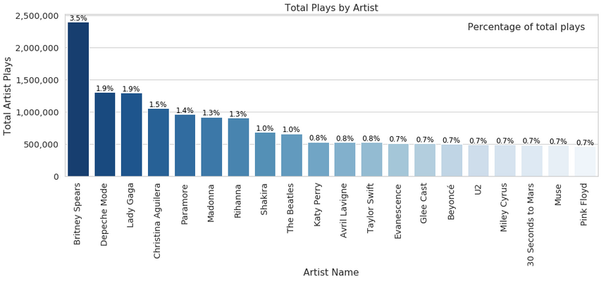
and the names of the artists that were played most:
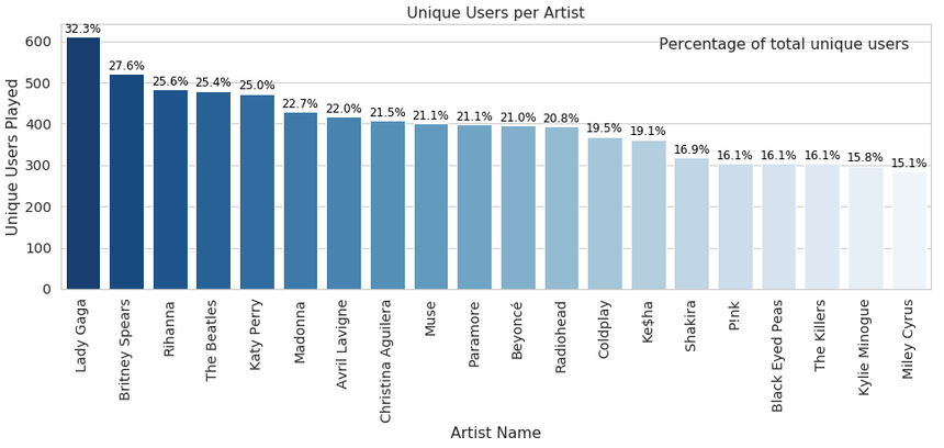
how much of the users play the artist:
here’s another look at artist popularity:
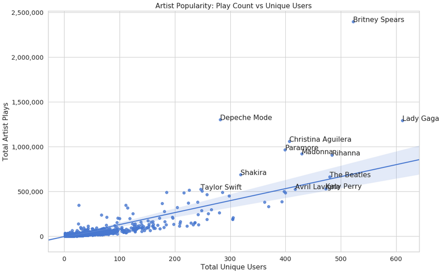
No surprises here, popular artists are taking the majority of the plays. Good thing that “The Beatles” still hold strong, though :)
Recommender Systems
Recommender systems (RS) are used pretty much everywhere where you have an array of items to choose from. They work by making suggestions that might help you make better/faster choices.
You might think that you’re a special snowflake, but RS exploit behavior patterns that are shared between users (you and other people). For example, you and your friends might have similar tastes for some stuff. RS try to find “friends” within other users and recommend things you haven’t tried that.
The two most used types of RS are Content-Based and Collaborative Filtering (CF). Collaborative filtering produces recommendations based on the knowledge of users’ preference to items, that is it uses the “wisdom of the crowd” to recommend items. In contrast, content-based recommender systems focus on the properties of the items and give you recommendations based on the similarity between them.
Collaborative Filtering (CF)
Collaborative filtering (CF) is the workhorse of recommender engines. What is good about the algorithm is its property of being able to do feature learning, which allows it to start to learn which features to use. CF can be divided into Memory-Based Collaborative Filtering and Model-Based Collaborative Filtering.
Memory-Based Collaborative Filtering
Memory-Based CF methods can be divided into two sections: user-item filtering and item-item filtering. Here is the difference:
- Item-Item Collaborative Filtering: “Users who liked this item also liked …”
- User-Item Collaborative Filtering: “Users who are similar to you (kinda like the twin you never knew you had) also liked …”
Both methods require user-item matrix that contain the ratings for user u for item i. From that, you can calculate the similarity matrix.
The similarity values in Item-Item Collaborative Filtering are calculated by taking into account all users who have rated a pair of items.
For User-Item Collaborative Filtering, the similarity values are calculated by observing all items that are rated by a pair of users.
Model-Based Collaborative Filtering
Model-based CF methods are based on matrix factorization (MF). MF methods are used as an unsupervised learning method for latent variable decomposition and dimensionality reduction. They can handle scalability and sparsity problems better than Memory-based CF.
The goal of MF is to learn latent user preferences and item attributes from known ratings. Then use those variable to predict unknown ratings through the dot product of the latent features of users and items.
Matrix factorization restructures the user-item matrix into a low-rank matrix. You can represent it by the multiplication of two low-rank matrices, where the rows contain a vector of latent variables. You want this matrix to approximate the original matrix, as closely as possible, by multiplying the low-rank matrices together. That way, you predict the missing entries in the original matrix.
Singular Value Decomposition
Collaborative Filtering can be formulated by approximating a matrix X by using Singular Value Decomposition (SVD). The winning team at the Netflix Prize competition used SVD matrix factorization models to win the prize. SVD can be expressed as:
X=USVTGiven m×n matrix X:
- U is (m×r) orthogonal matrix
- S is (r×r) diagonal matrix with non-negative real numbers on the diagonal
- VT is (r×n) orthogonal matrix
where U represents feature vectors of the users, V represents feature vectors of the items and the elements on the diagonal of S are known as singular values.
You can make a prediction by taking the dot product of U, S and VT. Here is a quick example of how you can implement SVD in Python:
1import scipy.sparse as sp2from scipy.sparse.linalg import svds34U, S, VT = svds(user_item_ratings, k = 20)5S_diagonal = np.diag(S)6Y_hat = np.dot(np.dot(U, S_diagonal), VT)Recommending music artists
While most tutorials on “the Internets” focus on memory-based approaches, they don’t seem to be used in practice. Although they produce good results, they do not scale well and suffer from the “cold-start” problem.
On the other hand, applying SVD requires factorization of the user-item matrix which can be expensive when the matrix is very sparse (lots of user-item ratings are missing). Also, imputing missing values is often used, since SVD doesn’t work when data is missing. This can significantly increase the amount of data and runtime performance of the algorithm.
More recent approaches have focused on predicting ratings by minimizing the regularized squared error with respect to a latent user feature matrix P and a latent item feature matrix Q:
Q∗,P∗min(u,i)∈K∑(rui−PuTQi)2+λ(∣∣Qi∣∣2+∣∣Pu∣∣2)Where K is a set of (u,i) pairs, r(u,i) is the rating for item i by user u and λ is a regularization term (used to avoid overfitting). The training of our model consists of minimizing the regularized squared error. After an estimate of P and Q is obtained, you can predict unknown ratings by taking the dot product of the latent features for users and items.
We can apply Stochastic Gradient Descent (SGD) or Alternating Least Squares (ALS) in order to minimize the loss function. Both methods can be used to incrementally update our model (online learning), as new rating comes in.
Here, we’ll implement SGD as it seems to be generally faster and more accurate than ALS (except in situations of highly sparse and implicit data). As an added bonus, SGD is widely used for training Deep Neural Networks (which we’ll discuss later). Thus, many high-quality implementations exist for this algorithm.
Preprocessing
In order to apply the CF algorithm, we need to transform our dataset into a user-artist play count matrix. Let’s do that after doing data scaling first:
1pc = ap.playCount2play_count_scaled = (pc - pc.min()) / (pc.max() - pc.min())34ap = ap.assign(playCountScaled=play_count_scaled)This squishes the play counts in the [0 - 1] range and adds a new column to our data frame. Let’s build our “ratings” data frame:
1ratings_df = ap.pivot(2 index='userID',3 columns='artistID',4 values='playCountScaled'5)67ratings = ratings_df.fillna(0).valuesWe use Pandas pivot method to create index / column data frame and fill the missing play counts with 0.
Let’s have a look at how sparse our data frame is:
1sparsity = float(len(ratings.nonzero()[0]))2sparsity /= (ratings.shape[0] * ratings.shape[1])3sparsity *= 1004print('{:.2f}%'.format(sparsity))10.28%Our dataset seems really sparse. Next, let’s split our data into training and validation data sets:
1train, val = train_test_split(ratings)Here, we define the train_test_split function a bit differently:
1MIN_USER_RATINGS = 352DELETE_RATING_COUNT = 1534def train_test_split(ratings):56 validation = np.zeros(ratings.shape)7 train = ratings.copy()89 for user in np.arange(ratings.shape[0]):10 if len(ratings[user,:].nonzero()[0]) >= MIN_USER_RATINGS:11 val_ratings = np.random.choice(12 ratings[user, :].nonzero()[0],13 size=DELETE_RATING_COUNT,14 replace=False15 )16 train[user, val_ratings] = 017 validation[user, val_ratings] = ratings[user, val_ratings]18 return train, validationOkay, that is a lot different than you might’ve expected. We remove some existing play counts from users by replacing them with zeros.
Measuring the error
One of the most popular metrics used to evaluate the accuracy of Recommender Systems is Root Mean Squared Error (RMSE), defined as:
RMSE=N1∑(yi−yi^)2where yi is the real value for item i, yi^ is the predicted one and N is the size of the training set.
A discussion on more evaluation metrics can be found here
Here is the RMSE in Python:
1def rmse(prediction, ground_truth):2 prediction = prediction[ground_truth.nonzero()].flatten()3 ground_truth = ground_truth[ground_truth.nonzero()].flatten()4 return sqrt(mean_squared_error(prediction, ground_truth))Training
Let’s use SGD to train our recommender:
1def fit(self, X_train, X_val):2 m, n = X_train.shape34 self.P = 3 * np.random.rand(self.n_latent_features, m)5 self.Q = 3 * np.random.rand(self.n_latent_features, n)67 self.train_error = []8 self.val_error = []910 users, items = X_train.nonzero()1112 for epoch in range(self.n_epochs):13 for u, i in zip(users, items):14 error = X_train[u, i] - self.predictions(self.P[:,u], self.Q[:,i])15 self.P[:, u] += self.learning_rate * \16 (error * self.Q[:, i] - self.lmbda * self.P[:, u])17 self.Q[:, i] += self.learning_rate * \18 (error * self.P[:, u] - self.lmbda * self.Q[:, i])1920 train_rmse = rmse(self.predictions(self.P, self.Q), X_train)21 val_rmse = rmse(self.predictions(self.P, self.Q), X_val)22 self.train_error.append(train_rmse)23 self.val_error.append(val_rmse)We start by creating 2 matrices for the latent features of the users and ratings. For each user, item pair, we calculate the error (note we use a simple difference of the existing and predicted ratings). We then update P and Q using Gradient Descent.
After each training epoch, we calculate the training and validation errors and store their values to analyze later. Here is the predictions method implementation:
1def predictions(self, P, Q):2 return np.dot(P.T, Q)As we discussed earlier, we obtain predictions by taking the dot product of the transposed P matrix with Q.
Evaluation
Let’s have a quick look at how the training process went by looking at the training and validation RMSE:
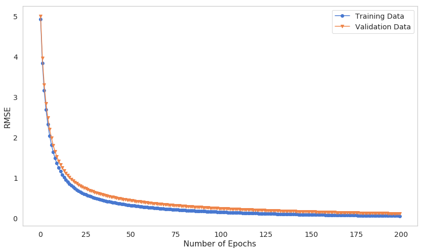
Our model seems to train gradually, and both errors decrease as the number of epochs increase. Note that you might want to spend even more time to train your model, as it might get even better.
Making recommendations
Finally, we are ready to make some recommendations for a user. Here is the implementation of the predict method:
1def predict(self, X_train, user_index):2 y_hat = self.predictions(self.P, self.Q)3 predictions_index = np.where(X_train[user_index, :] == 0)[0]4 return y_hat[user_index, predictions_index].flatten()First, we obtain the matrix with all predicted play counts. Second, we take the indices of all unknown play counts and return only these as predictions. Let’s make some recommendations for a specific user:
1user_id = 12362user_index = ratings_df.index.get_loc(user_id)3predictions_index = np.where(train[user_index, :] == 0)[0]45rating_predictions = recommender.predict(train, user_index)Before looking at the recommendation list, let’s have a look at what this user preferences currently are:
1existing_ratings_index = np.where(train[user_index, :] > 0)[0]2existing_ratings = train[user_index, existing_ratings_index]34create_artist_ratings(5 artists,6 existing_ratings_index,7 existing_ratings8)| name | rating |
|---|---|
| Marilyn Manson | 0.196486 |
| 3 Doors Down | 0.043204 |
| Pearl Jam | 0.042016 |
| Children of Bodom | 0.025657 |
| Disturbed | 0.021690 |
| Rammstein | 0.021562 |
| A Perfect Circle | 0.020879 |
| Gojira | 0.017051 |
| Rob Zombie | 0.016280 |
| D12 | 0.010990 |
And here are the recommendations from our model:
1create_artist_ratings(2 artists,3 predictions_index,4 rating_predictions5)| name | rating |
|---|---|
| Sander van Doorn | 0.559202 |
| Jacob Miller | 0.552893 |
| Celtas Cortos | 0.552142 |
| Camisa de Vênus | 0.546361 |
| Ella Fitzgerald & Louis Armstrong | 0.541477 |
| The Answer | 0.537367 |
| Anjelika Akbar | 0.536756 |
| Medications | 0.536486 |
| Lützenkirchen | 0.535515 |
| Archie Star | 0.535147 |
Now might be a good time to go on YouTube or Spotify and try out some of those artists!
Conclusion
Congratulations on building a highly performant Recommender System from scratch! You’ve learned how to:
- Prepare raw data for making recommendations
- Implemented a simple Stochastic Gradient Descent from scratch
- Used the model to make predictions for new artists you might actually enjoy!
Complete source code in Google Colaboratory Notebook
Can you apply this same model on your dataset? Tell me how it went in the comments below!
Share
Want to be a Machine Learning expert?
You'll never get spam from me