Curiousily

Object Detection on Custom Dataset with YOLO (v5) using PyTorch and Python

27.06.2020 — Deep Learning, Computer Vision, Object Detection, Neural Network, Python — 5 min read

TL;DR Learn how to build a custom dataset for YOLO v5 (darknet compatible) and use it to fine-tune a large object detection model. The model will be ready for real-time object detection on mobile devices.

In this tutorial, you’ll learn how to fine-tune a pre-trained YOLO v5 model for detecting and classifying clothing items from images.

Here’s what we’ll go over:

Install required libraries
Build a custom dataset in YOLO/darknet format
Learn about YOLO model family history
Fine-tune the largest YOLO v5 model
Evaluate the model
Look at some predictions

How good our final model is going to be?

Prerequisites

Let’s start by installing some required libraries by the YOLOv5 project:

1!pip install torch==1.5.1+cu101 torchvision==0.6.1+cu101 -f https://download.pytorch.org/whl/torch_stable.html
2!pip install numpy==1.17
3!pip install PyYAML==5.3.1
4!pip install git+https://github.com/cocodataset/cocoapi.git#subdirectory=PythonAPI

We’ll also install Apex by NVIDIA to speed up the training of our model (this step is optional):

1!git clone https://github.com/NVIDIA/apex && cd apex && pip install -v --no-cache-dir --global-option="--cpp_ext" --global-option="--cuda_ext" . --user && cd .. && rm -rf apex

Build a dataset

The dataset contains annotations for clothing items - bounding boxes around shirts, tops, jackets, sunglasses. The dataset is from DataTurks and is on Kaggle.

1!gdown --id 1uWdQ2kn25RSQITtBHa9_zayplm27IXNC

The dataset contains a single JSON file with URLs to all images and bounding box data.

Let’s import all required libraries:

1from pathlib import Path
2from tqdm import tqdm
3import numpy as np
4import json
5import urllib
6import PIL.Image as Image
7import cv2
8import torch
9import torchvision
10from IPython.display import display
11from sklearn.model_selection import train_test_split
12
13import seaborn as sns
14from pylab import rcParams
15import matplotlib.pyplot as plt
16from matplotlib import rc
17
18%matplotlib inline
19%config InlineBackend.figure_format='retina'
20sns.set(style='whitegrid', palette='muted', font_scale=1.2)
21rcParams['figure.figsize'] = 16, 10
22
23np.random.seed(42)

Each line in the dataset file contains a JSON object. Let’s create a list of all annotations:

1clothing = []
2with open("clothing.json") as f:
3    for line in f:
4        clothing.append(json.loads(line))

Here’s an example annotation:

1clothing[0]

1{'annotation': [{'imageHeight': 312,
2   'imageWidth': 147,
3   'label': ['Tops'],
4   'notes': '',
5   'points': [{'x': 0.02040816326530612, 'y': 0.2532051282051282},
6    {'x': 0.9931972789115646, 'y': 0.8108974358974359}]}],
7 'content': 'http://com.dataturks.a96-i23.open.s3.amazonaws.com/2c9fafb063ad2b650163b00a1ead0017/4bb8fd9d-8d52-46c7-aa2a-9c18af10aed6___Data_xxl-top-4437-jolliy-original-imaekasxahykhd3t.jpeg',
8 'extras': None}

We have the labels, image dimensions, bounding box points (normalized in 0-1 range), and an URL to the image file.

Do we have images with multiple annotations?

1for c in clothing:
2  if len(c['annotation']) > 1:
3    display(c)

1{'annotation': [{'imageHeight': 312,
2   'imageWidth': 265,
3   'label': ['Jackets'],
4   'notes': '',
5   'points': [{'x': 0, 'y': 0.6185897435897436},
6    {'x': 0.026415094339622643, 'y': 0.6185897435897436}]},
7  {'imageHeight': 312,
8   'imageWidth': 265,
9   'label': ['Skirts'],
10   'notes': '',
11   'points': [{'x': 0.01509433962264151, 'y': 0.03205128205128205},
12    {'x': 1, 'y': 0.9839743589743589}]}],
13 'content': 'http://com.dataturks.a96-i23.open.s3.amazonaws.com/2c9fafb063ad2b650163b00a1ead0017/b3be330c-c211-45bb-b244-11aef08021c8___Data_free-sk-5108-mudrika-original-imaf4fz626pegq9f.jpeg',
14 'extras': None}

Just a single example. We’ll need to handle it, though.

Let’s get all unique categories:

1categories = []
2for c in clothing:
3  for a in c['annotation']:
4    categories.extend(a['label'])
5categories = list(set(categories))
6categories.sort()
7categories

1['Jackets',
2     'Jeans',
3     'Shirts',
4     'Shoes',
5     'Skirts',
6     'Tops',
7     'Trousers',
8     'Tshirts',
9     'sunglasses']

We have 9 different categories. Let’s split the data into a training and validation set:

1train_clothing, val_clothing = train_test_split(clothing, test_size=0.1)
2len(train_clothing), len(val_clothing)

1(453, 51)

Sample image and annotation

Let’s have a look at an image from the dataset. We’ll start by downloading it:

1row = train_clothing[10]
2
3img = urllib.request.urlopen(row["content"])
4img = Image.open(img)
5img = img.convert('RGB')
6
7img.save("demo_image.jpeg", "JPEG")

Here’s how our sample annotation looks like:

1row

1{'annotation': [{'imageHeight': 312,
2   'imageWidth': 145,
3   'label': ['Tops'],
4   'notes': '',
5   'points': [{'x': 0.013793103448275862, 'y': 0.22756410256410256},
6    {'x': 1, 'y': 0.7948717948717948}]}],
7 'content': 'http://com.dataturks.a96-i23.open.s3.amazonaws.com/2c9fafb063ad2b650163b00a1ead0017/ec339ad6-6b73-406a-8971-f7ea35d47577___Data_s-top-203-red-srw-original-imaf2nfrxdzvhh3k.jpeg',
8 'extras': None}

We can use OpenCV to read the image:

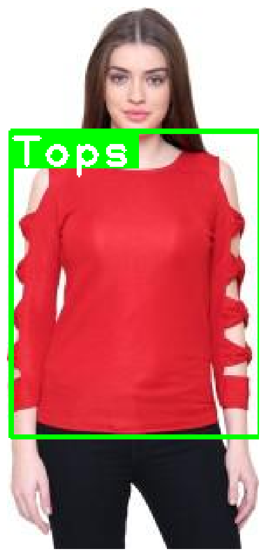
1img = cv2.cvtColor(cv2.imread(f'demo_image.jpeg'), cv2.COLOR_BGR2RGB)
2img.shape

1(312, 145, 3)

Let’s add the bounding box on top of the image along with the label:

1for a in row['annotation']:
2  for label in a['label']:
3
4    w = a['imageWidth']
5    h = a['imageHeight']
6
7    points = a['points']
8    p1, p2 = points
9
10    x1, y1 = p1['x'] * w, p1['y'] * h
11    x2, y2 = p2['x'] * w, p2['y'] * h
12
13    cv2.rectangle(
14      img,
15      (int(x1), int(y1)),
16      (int(x2), int(y2)),
17      color=(0, 255, 0),
18      thickness=2
19    )
20
21    ((label_width, label_height), _) = cv2.getTextSize(
22        label,
23        fontFace=cv2.FONT_HERSHEY_PLAIN,
24        fontScale=1.75,
25        thickness=2
26    )
27
28    cv2.rectangle(
29      img,
30      (int(x1), int(y1)),
31      (int(x1 + label_width + label_width * 0.05), int(y1 + label_height + label_height * 0.25)),
32      color=(0, 255, 0),
33      thickness=cv2.FILLED
34    )
35
36    cv2.putText(
37      img,
38      label,
39      org=(int(x1), int(y1 + label_height + label_height * 0.25)), # bottom left
40      fontFace=cv2.FONT_HERSHEY_PLAIN,
41      fontScale=1.75,
42      color=(255, 255, 255),
43      thickness=2
44    )

The point coordinates are converted back to pixels and used to draw rectangles over the image. Here’s the result:

1plt.imshow(img)
2plt.axis('off');

Convert to YOLO format

YOLO v5 requires the dataset to be in the darknet format. Here’s an outline of what it looks like:

One txt with labels file per image
One row per object
Each row contains: class_index bbox_x_center bbox_y_center bbox_width bbox_height
Box coordinates must be normalized between 0 and 1

Let’s create a helper function that builds a dataset in the correct format for us:

1def create_dataset(clothing, categories, dataset_type):
2
3  images_path = Path(f"clothing/images/{dataset_type}")
4  images_path.mkdir(parents=True, exist_ok=True)
5
6  labels_path = Path(f"clothing/labels/{dataset_type}")
7  labels_path.mkdir(parents=True, exist_ok=True)
8
9  for img_id, row in enumerate(tqdm(clothing)):
10
11    image_name = f"{img_id}.jpeg"
12
13    img = urllib.request.urlopen(row["content"])
14    img = Image.open(img)
15    img = img.convert("RGB")
16
17    img.save(str(images_path / image_name), "JPEG")
18
19    label_name = f"{img_id}.txt"
20
21    with (labels_path / label_name).open(mode="w") as label_file:
22
23      for a in row['annotation']:
24
25        for label in a['label']:
26
27          category_idx = categories.index(label)
28
29          points = a['points']
30          p1, p2 = points
31
32          x1, y1 = p1['x'], p1['y']
33          x2, y2 = p2['x'], p2['y']
34
35          bbox_width = x2 - x1
36          bbox_height = y2 - y1
37
38          label_file.write(
39            f"{category_idx} {x1 + bbox_width / 2} {y1 + bbox_height / 2} {bbox_width} {bbox_height}\n"
40          )

We’ll use it to create the train and validation datasets:

1create_dataset(train_clothing, categories, 'train')
2create_dataset(val_clothing, categories, 'val')

Let’s have a look at the file structure:

1!tree clothing -L 2

1clothing
2├── images
3│   ├── train
4│   └── val
5└── labels
6├── train
7└── val
8
96 directories, 0 files

And a single annotation example:

1!cat clothing/labels/train/0.txt

14 0.525462962962963 0.5432692307692308 0.9027777777777778 0.9006410256410257

Fine-tuning YOLO v5

The YOLO abbreviation stands for You Only Look Once. YOLO models are one stage object detectors.

One-stage vs two-stage object detectors. Image from the YOLO v4 paper

YOLO models are very light and fast. They are not the most accurate object detections around, though. Ultimately, those models are the choice of many (if not all) practitioners interested in real-time object detection (FPS >30).

Contreversy

Joseph Redmon introduced YOLO v1 in the 2016 paper You Only Look Once: Unified, Real-Time Object Detection. The implementation uses the Darknet Neural Networks library.

He also co-authored the YOLO v2 paper in 2017 YOLO9000: Better, Faster, Stronger. A significant improvement over the first iteration with much better localization of objects.

The final iteration, from the original author, was published in the 2018 paper YOLOv3: An Incremental Improvement.

Then things got a bit wacky. Alexey Bochkovskiy published YOLOv4: Optimal Speed and Accuracy of Object Detection on April 23, 2020. The project has an open-source repository on GitHub.

YOLO v5 got open-sourced on May 30, 2020 by Glenn Jocher from ultralytics. There is no published paper, but the complete project is on GitHub.

The community at Hacker News got into a heated debate about the project naming. Even the guys at Roboflow wrote Responding to the Controversy about YOLOv5 article about it. They also did a great comparison between YOLO v4 and v5.

My opinion? As long as you put out your work for the whole world to use/see - I don’t give a flying fuck. I am not going to comment on points/arguments that are obvious.

YOLO v5 project setup

YOLO v5 uses PyTorch, but everything is abstracted away. You need the project itself (along with the required dependencies).

Let’s start by cloning the GitHub repo and checking out a specific commit (to ensure reproducibility):

1!git clone https://github.com/ultralytics/yolov5
2%cd yolov5
3!git checkout ec72eea62bf5bb86b0272f2e65e413957533507f

We need two configuration files. One for the dataset and one for the model we’re going to use. Let’s download them:

1!gdown --id 1ZycPS5Ft_0vlfgHnLsfvZPhcH6qOAqBO -O data/clothing.yaml
2!gdown --id 1czESPsKbOWZF7_PkCcvRfTiUUJfpx12i -O models/yolov5x.yaml

The model config changes the number of classes to 9 (equal to the ones in our dataset). The dataset config clothing.yaml is a bit more complex:

1train: ../clothing/images/train/
2val: ../clothing/images/val/
3
4nc: 9
5
6names:
7  [
8    "Jackets",
9    "Jeans",
10    "Shirts",
11    "Shoes",
12    "Skirts",
13    "Tops",
14    "Trousers",
15    "Tshirts",
16    "sunglasses",
17  ]

This file specifies the paths to the training and validation sets. It also gives the number of classes and their names (you should order those correctly).

Training

Fine-tuning an existing model is very easy. We’ll use the largest model YOLOv5x (89M parameters), which is also the most accurate.

In our case, we don’t really care about speed. We just want the best accuracy you can get. The checkpoint you’re going to use for a different problem(s) is contextually specific. Take a look at the overview of the pre-trained checkpoints.

To train a model on a custom dataset, we’ll call the train.py script. We’ll pass a couple of parameters:

img 640 - resize the images to 640x640 pixels
batch 4 - 4 images per batch
epochs 30 - train for 30 epochs
data ./data/clothing.yaml - path to dataset config
cfg ./models/yolov5x.yaml - model config
weights yolov5x.pt - use pre-trained weights from the YOLOv5x model
name yolov5x_clothing - name of our model
cache - cache dataset images for faster training

1!python train.py --img 640 --batch 4 --epochs 30 \
2  --data ./data/clothing.yaml --cfg ./models/yolov5x.yaml --weights yolov5x.pt \
3  --name yolov5x_clothing --cache

The training took around 30 minutes on Tesla P100. The best model checkpoint is saved to weights/best_yolov5x_clothing.pt.

Evaluation

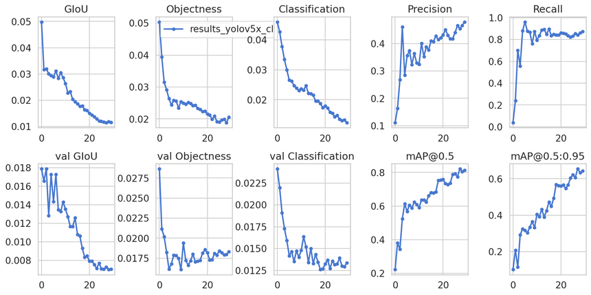
The project includes a great utility function plot_results() that allows you to evaluate your model performance on the last training run:

1from utils.utils import plot_results
2
3plot_results();

Looks like the mean average precision (mAP) is getting better throughout the training. The model might benefit from more training, but it is good enough.

Making predictions

Let’s pick 50 images from the validation set and move them to inference/images to see how our model does on those:

1!find ../clothing/images/val/ -maxdepth 1 -type f | head -50 | xargs cp -t "./inference/images/"

We’ll use the detect.py script to run our model on the images. Here are the parameters we’re using:

weights weights/best_yolov5x_clothing.pt - checkpoint of the model
img 640 - resize the images to 640x640 px
conf 0.4 - take into account predictions with confidence of 0.4 or higher
source ./inference/images/ - path to the images

1!python detect.py --weights weights/best_yolov5x_clothing.pt \
2  --img 640 --conf 0.4 --source ./inference/images/

We’ll write a helper function to show the results:

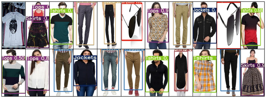
1def load_image(img_path: Path, resize=True):
2  img = cv2.cvtColor(cv2.imread(str(img_path)), cv2.COLOR_BGR2RGB)
3  img = cv2.resize(img, (128, 256), interpolation = cv2.INTER_AREA)
4  return img
5
6def show_grid(image_paths):
7  images = [load_image(img) for img in image_paths]
8  images = torch.as_tensor(images)
9  images = images.permute(0, 3, 1, 2)
10  grid_img = torchvision.utils.make_grid(images, nrow=11)
11  plt.figure(figsize=(24, 12))
12  plt.imshow(grid_img.permute(1, 2, 0))
13  plt.axis('off');

Here are some of the images along with the detected clothing:

1img_paths = list(Path("inference/output").glob("*.jpeg"))[:22]
2show_grid(img_paths)

To be honest with you. I am really blown away with the results!

Summary

You now know how to create a custom dataset and fine-tune one of the YOLO v5 models on your own. Nice!

Here’s what you’ve learned:

Install required libraries
Build a custom dataset in YOLO/darknet format
Learn about YOLO model family history
Fine-tune the largest YOLO v5 model
Evaluate the model
Look at some predictions

How well does your model do on your dataset? Let me know in the comments below.

In the next part, you’ll learn how to deploy your model a mobile device.

References

Want to be a Machine Learning expert?

Join the weekly newsletter on Data Science, Deep Learning and Machine Learning in your inbox, curated by me! Chosen by 10,000+ Machine Learning practitioners. (There might be some exclusive content, too!)

You'll never get spam from me

Hacker's Guide to Neural Networks in JavaScript

Build Machine Learning models (especially Deep Neural Networks) that you can easily integrate with existing or new web apps. Think of your ReactJs, Vue, or Angular app enhanced with the power of Machine Learning models.

Get SH*T Done with PyTorch

Learn how to solve real-world problems with Deep Learning models (NLP, Computer Vision, and Time Series). Go from prototyping to deployment with PyTorch and Python!

Hacker's Guide to Machine Learning with Python

This book brings the fundamentals of Machine Learning to you, using tools and techniques used to solve real-world problems in Computer Vision, Natural Language Processing, and Time Series analysis. The skills taught in this book will lay the foundation for you to advance your journey to Machine Learning Mastery!

Hands-On Machine Learning from Scratch

This book will guide you on your journey to deeper Machine Learning understanding by developing algorithms in Python from scratch! Learn why and when Machine learning is the right tool for the job and how to improve low performing models!