TL;DR Build a Linear Regression model in TensorFlow.js to predict house prices. Learn how to handle categorical data and do feature scaling.

Raining again. It has been 3 weeks since the last time you saw the sun. You’re getting tired of all this cold and unpleasant feeling of loneliness and melancholy.

The voice in your head is getting louder and louder.

- “MOVE”.

Alright, you’re ready to do it. Where to? You remember that you’re nearly broke.

A friend of yours told you about this place Ames, Iowa and it stuck in your head. After a quick search, you found that the weather is pleasant during the year and there is some rain, but not much. Excitement!

Fortunately, you know of this dataset on Kaggle that might help you find out how much your dream house might cost. Let’s get to it!

Run the complete source code for this tutorial right in your browser:

House prices data

Our data comes from Kaggle’s House Prices: Advanced Regression Techniques challenge.

With 79 explanatory variables describing (almost) every aspect of residential homes in Ames, Iowa, this competition challenges you to predict the final price of each home.

Here’s a subset of the data we’re going to use for our model:

• OverallQual - Rates the overall material and finish of the house (0 - 10)
• GrLivArea - Above grade (ground) living area square feet
• GarageCars - Size of garage in car capacity
• TotalBsmtSF - Total square feet of basement area
• FullBath - Full bathrooms above grade
• YearBuilt - Original construction date
• SalePrice - The property’s sale price in dollars (we’re trying to predict this)

Let’s use Papa Parse to load the training data:

1const prepareData = async () => {
2  const csv = await Papa.parsePromise(
3    "https://raw.githubusercontent.com/curiousily/Linear-Regression-with-TensorFlow-js/master/src/data/housing.csv"
4  )
5
6  return csv.data
7}

1const data = await prepareData()

Exploration

Let’s build a better understanding of our data. First - the quality score of each house:

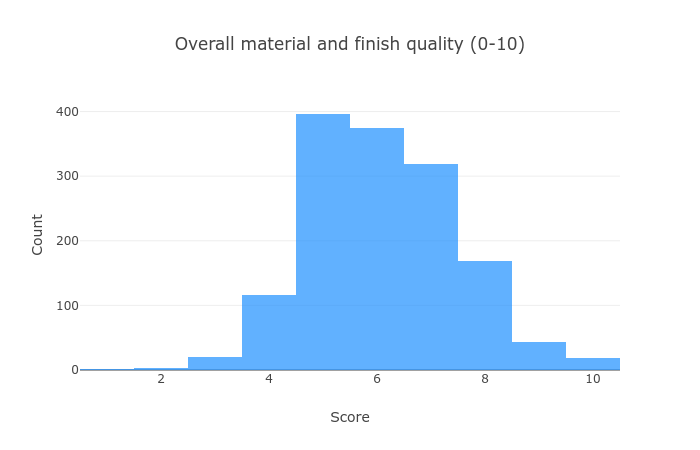
Most houses are of average quality, but there are more “good” than “bad” ones.

Let’s see how large are they (that’s what she said):

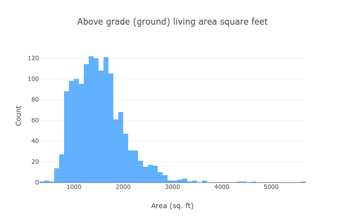
Most of the houses are within the 1,000 - 2,000 range, and we have some that are bigger.

Let’s have a look at the year they are built:

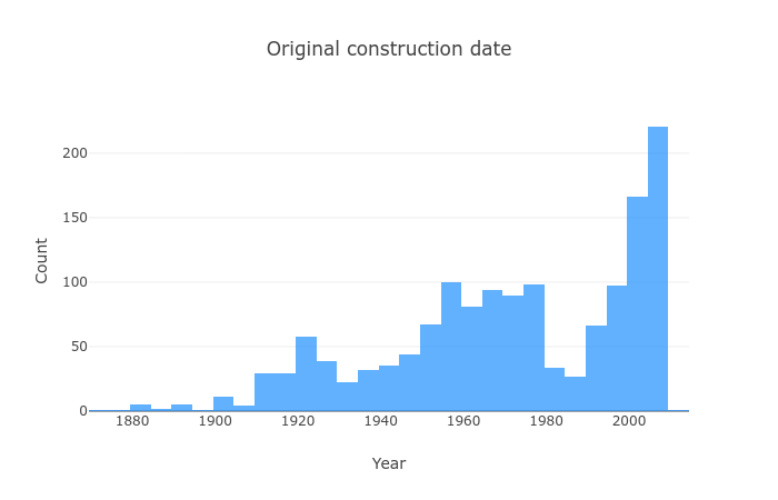
Even though there are a lot of houses that were built recently, we have a much more widespread distribution.

How related is the year with the price?

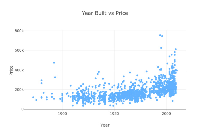
Seems like newer houses are pricier, no love for the old and well made then?

Oh ok, but higher quality should equal higher price, right?

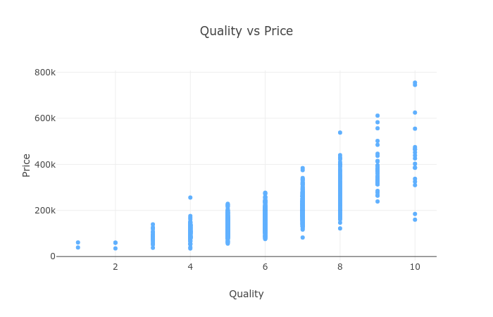
Generally yes, but look at quality 10. Some of those are relatively cheap. Any ideas why that might be?

Is a larger house equal higher price?

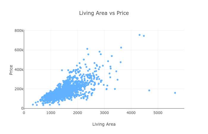
Seems like it, we might start our price prediction model using the living area!

Linear Regression

Linear Regression models assume that there is a linear relationship (can be modeled using a straight line) between a dependent continuous variable $Y$ and one or more explanatory (independent) variables $X$.

In our case, we’re going to use features like living area (X) to predict the sale price (Y) of a house.

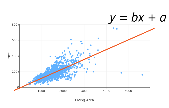
Simple Linear Regression

Simple Linear Regression is a model that has a single independent variable $X$. It is given by:

Where a and b are parameters, learned during the training of our model. $X$ is the data we’re going to use to train our model, $b$ controls the slope and $a$ the interception point with the $y$ axis.

Multiple Linear Regression

A natural extension of the Simple Linear Regression model is the multivariate one. It is given by:

where $x_1, x_2 \ldots, x_n$ are features from our dataset and $w_1, w_2 \ldots, w_n$ are learned parameters.

Loss function

We’re going to use Root Mean Squared Error to measure how far our predictions are from the real house prices. It is given by:

where the hypothesis/prediction $h_w$ is given by:

Data Preprocessing

Currently, our data sits into an array of JS objects. We need to turn it into Tensors and use it for training our model(s). Here is the code for that:

1const createDataSets = (data, features, categoricalFeatures, testSize) => {
2  const X = data.map(r =>
3    features.flatMap(f => {
4      if (categoricalFeatures.has(f)) {
5        return oneHot(!r[f] ? 0 : r[f], VARIABLE_CATEGORY_COUNT[f])
6      }
7      return !r[f] ? 0 : r[f]
8    })
9  )
10
11  const X_t = normalize(tf.tensor2d(X))
12
13  const y = tf.tensor(data.map(r => (!r.SalePrice ? 0 : r.SalePrice)))
14
15  const splitIdx = parseInt((1 - testSize) * data.length, 10)
16
17  const [xTrain, xTest] = tf.split(X_t, [splitIdx, data.length - splitIdx])
18  const [yTrain, yTest] = tf.split(y, [splitIdx, data.length - splitIdx])
19
20  return [xTrain, xTest, yTrain, yTest]
21}

We store our features in X and the labels in y. Then we convert the data into Tensors and split it into training and testing datasets.

Categorical features

Some of the features in our dataset are categorical/enumerable. For example, GarageCars can be in the 0-5 range.

Leaving categories represented as integers in our dataset might introduce implicit ordering dependence. Something that does not exist with categorical variables.

We’ll use one-hot encoding from TensorFlow to create an integer vector for each value to break the ordering. First, let’s specify how many different values each category has:

1const VARIABLE_CATEGORY_COUNT = {
2  OverallQual: 10,
3  GarageCars: 5,
4  FullBath: 4,
5}

We’ll use tf.oneHot() to convert individual value to a one-hot representation:

1const oneHot = (val, categoryCount) =>
2  Array.from(tf.oneHot(val, categoryCount).dataSync())

Note that the createDataSets() function accepts a parameter called categoricalFeatures which should be a set. We’ll use this to check whether or not we should process this feature as categorical.

Feature scaling

Feature scaling is used to transform the feature values into a (similar) range. Feature scaling will help our model(s) learn faster since we’re using Gradient Descent for training it.

Let’s use one of the simplest method for feature scaling - min-max normalization:

1const normalize = tensor =>
2  tf.div(tf.sub(tensor, tf.min(tensor)), tf.sub(tf.max(tensor), tf.min(tensor)))

this method rescales the range of values in the range of [0, 1].

Predicting house prices

Now that we know about the Linear Regression model(s), we can try to predict house prices based on the data we have. Let’s start simple:

Building a Simple Linear Regression model

We’ll wrap the training process in a function that we can reuse for our future model(s):

1const trainLinearModel = async (xTrain, yTrain) => {
2  ...
3}

trainLinearModel accepts the features and labels for our model. Let’s define a Linear Regression model using TensorFlow:

1const model = tf.sequential()
2
3model.add(
4  tf.layers.dense({
5    inputShape: [xTrain.shape[1]],
6    units: xTrain.shape[1],
7  })
8)
9
10model.add(tf.layers.dense({ units: 1 }))

Since TensorFlow.js doesn’t offer RMSE loss function, we’ll use MSE and take the square root of that later. We’ll also track Mean Absolute Error (MAE) between the predictions and real prices:

1model.compile({
2  optimizer: tf.train.sgd(0.001),
3  loss: "meanSquaredError",
4  metrics: [tf.metrics.meanAbsoluteError],
5})

Here’s the training process:

1const trainLogs = []
2const lossContainer = document.getElementById("loss-cont")
3const accContainer = document.getElementById("acc-cont")
4
5await model.fit(xTrain, yTrain, {
6  batchSize: 32,
7  epochs: 100,
8  shuffle: true,
9  validationSplit: 0.1,
10  callbacks: {
11    onEpochEnd: async (epoch, logs) => {
12      trainLogs.push({
13        rmse: Math.sqrt(logs.loss),
14        val_rmse: Math.sqrt(logs.val_loss),
15        mae: logs.meanAbsoluteError,
16        val_mae: logs.val_meanAbsoluteError,
17      })
18      tfvis.show.history(lossContainer, trainLogs, ["rmse", "val_rmse"])
19      tfvis.show.history(accContainer, trainLogs, ["mae", "val_mae"])
20    },
21  },
22})

We train for 100 epochs, shuffle the data beforehand, and use 10% of it for validation. The RMSE and MAE are visualized after each epoch.

Training

Our Simple Linear Regression model is using the GrLivArea feature:

1const [xTrainSimple, xTestSimple, yTrainSimple, yTestIgnored] = createDataSets(
2  data,
3  ["GrLivArea"],
4  new Set(),
5  0.1
6)
7
8const simpleLinearModel = await trainLinearModel(xTrainSimple, yTrainSimple)

We don’t have categorical features, so we leave that set is empty. Let’s have a look at the performance:

Building a Multiple Linear Regression model

We have a lot more data we haven’t used yet. Let’s see if that will help improve the predictions:

1const features = [
2  "OverallQual",
3  "GrLivArea",
4  "GarageCars",
5  "TotalBsmtSF",
6  "FullBath",
7  "YearBuilt",
8]
9
10const categoricalFeatures = new Set(["OverallQual", "GarageCars", "FullBath"])
11
12const [xTrain, xTest, yTrain, yTest] = createDataSets(
13  data,
14  features,
15  categoricalFeatures,
16  0.1
17)

We use all features in our dataset and pass a set of the categorical ones. Did we do better?

Overall, both models are performing at about the same level. This time, increasing the model complexity didn’t give us better accuracy.

Evaluation

Another way to evaluate our models is to check their predictions against the test data. Let’s start with the Simple Linear Regression:

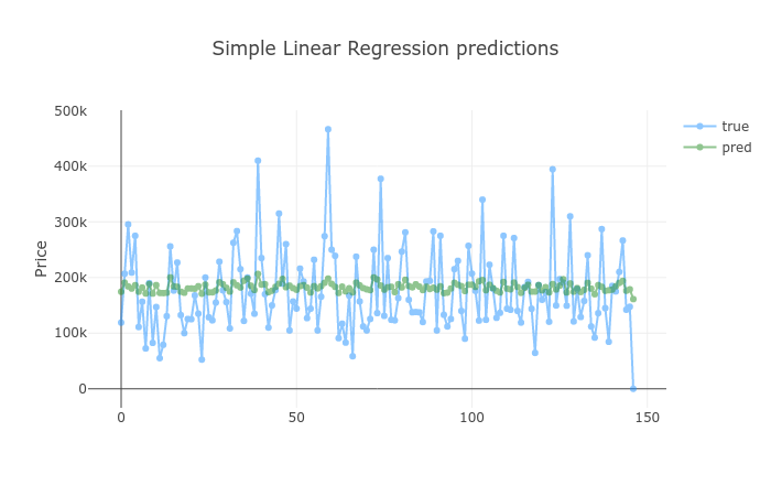
How did adding more data improved the predictions?

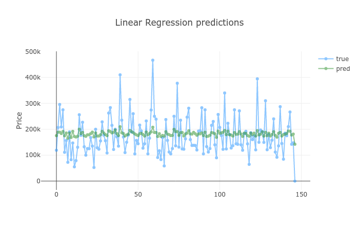
Well, it didn’t. Again, having a more complex model trained with more data didn’t provide better performance.

Conclusion

You did it! You built two Linear Regression models that predict house price based on a set of features. You also did:

• Feature scaling for faster model training
• Convert categorical variables into one-hot representations
• Implement RMSE (based on MSE) for accuracy evaluation

Run the complete source code for this tutorial right in your browser:

Is it time to learn about Neural Networks?

References

Handling Categorical Data in Machine Learning Models

About Feature Scaling and Normalization

RMSE: Root Mean Square Error