Predicting House Prices with Linear Regression | Machine Learning from Scratch (Part II)
— Machine Learning, Statistics, Linear Regression — 4 min read
Share
TL;DR Use a test-driven approach to build a Linear Regression model using Python from scratch. You will use your trained model to predict house sale prices and extend it to a multivariate Linear Regression.
I know that you’ve always dreamed of dominating the housing market. Until now, that was impossible. But with this limited offer you can… got a bit sidetracked there.
Let’s start building our model with Python, but this time we will use it on a more realistic dataset.
Complete source code notebook on Google Colaboratory
The Data
Our data comes from a Kaggle competition named “House Prices: Advanced Regression Techniques”. It contains 1460 training data points and 80 features that might help us predict the selling price of a house.
Load the data
Let’s load the Kaggle dataset into a Pandas data frame:
1df_train = pd.read_csv('house_prices_train.csv')Exploration — getting a feel for our data
We’re going to predict the SalePrice column ($ USD), let’s start with it:
1count 1460.0000002mean 180921.1958903std 79442.5028834min 34900.000000525% 129975.000000650% 163000.000000775% 214000.0000008max 755000.0000009Name: SalePrice, dtype: float64
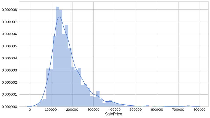
Most of the density lies between 100k and 250k, but there appears to be a lot of outliers on the pricier side.
Next, let’s have a look at the greater living area (square feet) against the sale price:
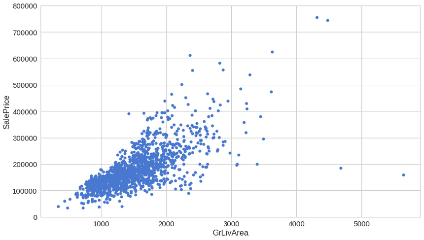
You might’ve expected that larger living area should mean a higher price. This chart shows you’re generally correct. But what are those 2–3 “cheap” houses offering huge living area?
One column you might not think about exploring is the TotalBsmtSF — Total square feet of the basement area, but let’s do it anyway:
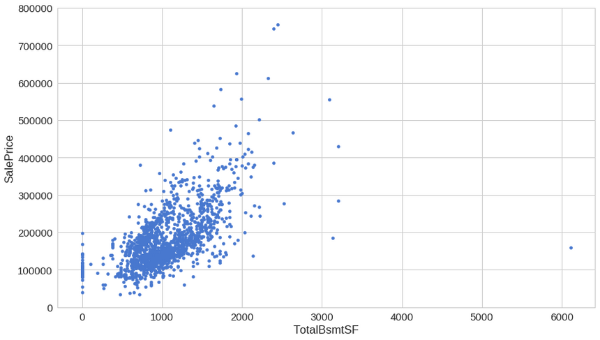
Intriguing, isn’t it? The basement area seems like it might have a lot of predictive power for our model.
Ok, last one. Let’s look at “OverallQual” — overall material and finish quality. Of course, this one seems like a much more subjective feature, so it might provide a bit different perspective on the sale price.
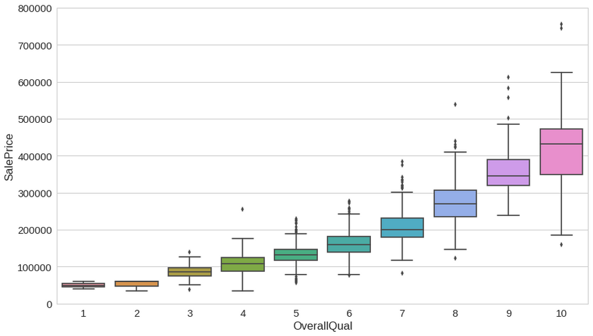
Everything seems fine for this one, except that when you look to the right things start getting much more nuanced. Will that “confuse” our model?
Let’s have a more general view on the top 8 correlated features with the sale price:
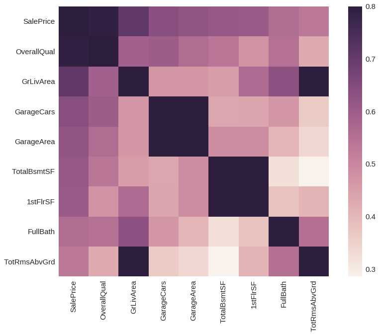
Surprised? All the features we discussed so far appear to be present. Its almost like we knew them from the start…
Do we have missing data?
We still haven’t discussed ways to “handle” missing data, so we’ll handle them like a boss — just not use those features:
| Row count | Percentage | |
|---|---|---|
| PoolQC | 1453 | 0.995205 |
| MiscFeature | 1406 | 0.963014 |
| Alley | 1369 | 0.937671 |
| Fence | 1179 | 0.807534 |
| FireplaceQu | 690 | 0.472603 |
| LotFrontage | 259 | 0.177397 |
| GarageCond | 81 | 0.055479 |
| GarageType | 81 | 0.055479 |
| GarageYrBlt | 81 | 0.055479 |
| GarageFinish | 81 | 0.055479 |
| GarageQual | 81 | 0.055479 |
| BsmtExposure | 38 | 0.026027 |
| BsmtFinType2 | 38 | 0.026027 |
| BsmtFinType1 | 37 | 0.025342 |
| BsmtCond | 37 | 0.025342 |
Yes, we’re not going to use any of those.
Predicting the sale price
Now that we have some feel of the data we’re playing with we can start our plan of attack — how to predict the sale price for a given house?
Using Linear Regression
 source: http://mybooksucks.com
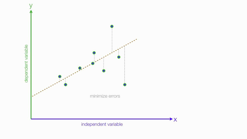
Linear regression models assume that the relationship between a dependent continuous variable Y and one or more explanatory (independent) variables X is linear (that is, a straight line).
It’s used to predict values within a continuous range (e.g. sales, price) rather than trying to classify them into categories (e.g. cat, dog). Linear regression models can be divided into two main types:
Simple Linear Regression
Simple linear regression uses a traditional slope-intercept form, where a and b are the coefficients that we try to “learn” and produce the most accurate predictions. X represents our input data and Y is our prediction.
Y=bX+a
 source: https://spss-tutorials.com
Multivariable Regression
A more complex, multi-variable linear equation might look like this, where w represents the coefficients or weights, our model will try to learn.
Y(x1,x2,x3)=w1x1+w2x2+w3x3+w0The variables x1,x2,x3 represent the attributes or distinct pieces of information, we have about each observation.
Loss function
Given our Simple Linear Regression equation:
Y=bX+aWe can use the following cost function to find the coefficients/parameters for our model:
Mean Squared Error (MSE) Cost Function
The MSE is defined as:
MSE=J(W)=m1i=1∑m(y(i)−hw(x(i)))2where
hw(x)=g(wTx)The MSE measures how much the average model predictions vary from the correct values. The number is higher when the model is performing “bad” on our training data.
The first derivative of MSE is given by:
MSE′=J′(W)=m2i=1∑m(hw(x(i))−y(i))One Half Mean Squared Error (OHMSE)
We will apply a small modification to the MSE — multiply by 21 so when we take the derivative, the 2s cancel out:
OHMSE=J(W)=2m1i=1∑m(y(i)−hw(x(i)))2The first derivative of OHMSE is given by:
OHMSE′=J′(W)=m1i=1∑m(hw(x(i))−y(i))Let’s implement it in Python (yes, we’re going TDD style!)
1class TestLoss(unittest.TestCase):23 def test_zero_h_zero_y(self):4 self.assertAlmostEqual(loss(h=np.array([0]), y=np.array([0])), 0)56 def test_one_h_zero_y(self):7 self.assertAlmostEqual(loss(h=np.array([1]), y=np.array([0])), 0.5)89 def test_two_h_zero_y(self):10 self.assertAlmostEqual(loss(h=np.array([2]), y=np.array([0])), 2)1112 def test_zero_h_one_y(self):13 self.assertAlmostEqual(loss(h=np.array([0]), y=np.array([1])), 0.5)1415 def test_zero_h_two_y(self):16 self.assertAlmostEqual(loss(h=np.array([0]), y=np.array([2])), 2)Now that we have the tests ready, we can implement the loss function:
1def loss(h, y):2 sq_error = (h - y)**23 n = len(y)4 return 1.0 / (2*n) * sq_error.sum()1run_tests()time for the results:
1.....23--------------------------------------------------------------4Ran 5 tests in 0.007s5OKData preprocessing
We will do a little preprocessing to our data using the following formula (standardization):
x′=σx−μwhere μ is the population mean and σ is the standard deviation.
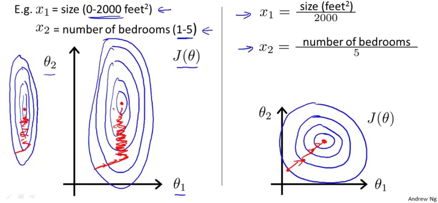
But why? Why would we want to do that? The following chart might help you out:
 source: Andrew Ng
What the doodle shows us that our old friend — the gradient descent algorithm, might converge (find good parameters) faster when our training data is scaled. Shall we?
1x = df_train['GrLivArea']2y = df_train['SalePrice']34x = (x - x.mean()) / x.std()5x = np.c_[np.ones(x.shape[0]), x]We will only use the greater living area feature for our first model.
Implementing Linear Regression
First, our tests:
1class TestLinearRegression(unittest.TestCase):23 def test_find_coefficients(self):4 clf = LinearRegression()5 clf.fit(x, y, n_iter=2000, lr=0.01)6 np.testing.assert_array_almost_equal(7 clf._W,8 np.array([180921.19555322, 56294.90199925])9 )Without further ado, the simple linear regression implementation:
1class LinearRegression:23 def predict(self, X):4 return np.dot(X, self._W)56 def _gradient_descent_step(self, X, targets, lr):78 predictions = self.predict(X)910 error = predictions - targets11 gradient = np.dot(X.T, error) / len(X)1213 self._W -= lr * gradient1415 def fit(self, X, y, n_iter=100000, lr=0.01):1617 self._W = np.zeros(X.shape[1])1819 for i in range(n_iter):20 self._gradient_descent_step(x, y, lr)2122 return selfYou might find our Linear Regression implementation simpler compared to the one presented for the Logistic Regression. Note that the use of the Gradient Descent algorithm is pretty much the same. Interesting, isn’t it? A single algorithm can build two different types of models. Would we be able to use it for more?
1run_tests()1......23-------------------------------------- Ran 6 tests in 1.094s4OKPredicting the sale price with our first model
Let’s use our freshly created model to begin our housing market domination:
1clf = LinearRegression()2clf.fit(x, y, n_iter=2000, lr=0.01)So how did the training go?
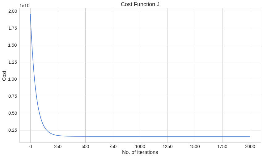
Our cost, at the last iteration, has a value of:
11569921604.8332634Can we do better?
Multivariable Linear Regression
Let’s use more of the available data to build a Multivariable Linear Regression model and see whether or not that will improve our OHMSE error. Let’s not forget that scaling too:
1x = df_train[['OverallQual', 'GrLivArea', 'GarageCars']]23x = (x - x.mean()) / x.std()4x = np.c_[np.ones(x.shape[0]), x]Implementing Multivariable Linear Regression
This space is intentionally left (kinda) blank
Using Multivariable Linear Regression
Now that the implementation of our new model is done, we can use it. Done!?
You see, young padawan, the magical world of software development has those mythical creates called abstractions. While it might be extraordinarily hard to get them right, they might reduce the complexity of the code you write by (pretty much) a ton.
You just used one such abstraction — called vectorization. Essentially, that allowed us to build a Multivariable Linear Regression model without the need to loop over all features in our dataset. Neat, right?
Our client interface stays the same, too:
1clf = LinearRegression()2clf.fit(x, y, n_iter=2000, lr=0.01)And the results:
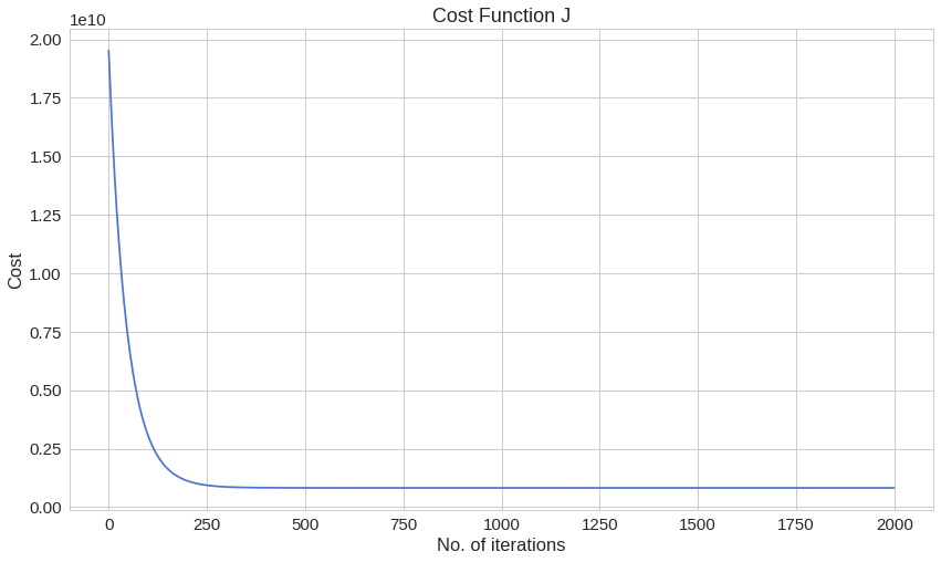
1822817042.8437098The loss at the last iteration is nearly 2 times smaller. Does this mean that our model is better now?
Complete source code notebook on Google Colaboratory
Conclusion
Nice! You just implemented a Linear Regression model and not the simple/crappy kind.
One thing you might want to try is to predict house sale prices on the testing dataset from Kaggle. Is this model any good on it?
In the next part, you’re going to implement a Decision Tree model from scratch!
Share
Want to be a Machine Learning expert?
You'll never get spam from me