Curiousily

Sentiment Analysis with BERT and Transformers by Hugging Face using PyTorch and Python

20.04.2020 — Deep Learning, NLP, Machine Learning, Neural Network, Sentiment Analysis, Python — 7 min read

TL;DR In this tutorial, you’ll learn how to fine-tune BERT for sentiment analysis. You’ll do the required text preprocessing (special tokens, padding, and attention masks) and build a Sentiment Classifier using the amazing Transformers library by Hugging Face!

You’ll learn how to:

Intuitively understand what BERT is
Preprocess text data for BERT and build PyTorch Dataset (tokenization, attention masks, and padding)
Use Transfer Learning to build Sentiment Classifier using the Transformers library by Hugging Face
Evaluate the model on test data
Predict sentiment on raw text

Let’s get started!

What is BERT?

BERT (introduced in this paper) stands for Bidirectional Encoder Representations from Transformers. If you don’t know what most of that means - you’ve come to the right place! Let’s unpack the main ideas:

Bidirectional - to understand the text you’re looking you’ll have to look back (at the previous words) and forward (at the next words)
Transformers - The Attention Is All You Need paper presented the Transformer model. The Transformer reads entire sequences of tokens at once. In a sense, the model is non-directional, while LSTMs read sequentially (left-to-right or right-to-left). The attention mechanism allows for learning contextual relations between words (e.g. his in a sentence refers to Jim).
(Pre-trained) contextualized word embeddings - The ELMO paper introduced a way to encode words based on their meaning/context. Nails has multiple meanings - fingernails and metal nails.

BERT was trained by masking 15% of the tokens with the goal to guess them. An additional objective was to predict the next sentence. Let’s look at examples of these tasks:

Masked Language Modeling (Masked LM)

The objective of this task is to guess the masked tokens. Let’s look at an example, and try to not make it harder than it has to be:

That’s [mask] she [mask] -> That’s what she said

Next Sentence Prediction (NSP)

Given a pair of two sentences, the task is to say whether or not the second follows the first (binary classification). Let’s continue with the example:

Input = [CLS] That’s [mask] she [mask]. [SEP] Hahaha, nice! [SEP]

Label = IsNext

Input = [CLS] That’s [mask] she [mask]. [SEP] Dwight, you ignorant [mask]! [SEP]

Label = NotNext

The training corpus was comprised of two entries: Toronto Book Corpus (800M words) and English Wikipedia (2,500M words). While the original Transformer has an encoder (for reading the input) and a decoder (that makes the prediction), BERT uses only the decoder.

BERT is simply a pre-trained stack of Transformer Encoders. How many Encoders? We have two versions - with 12 (BERT base) and 24 (BERT Large).

Is This Thing Useful in Practice?

The BERT paper was released along with the source code and pre-trained models.

The best part is that you can do Transfer Learning (thanks to the ideas from OpenAI Transformer) with BERT for many NLP tasks - Classification, Question Answering, Entity Recognition, etc. You can train with small amounts of data and achieve great performance!

Setup

We’ll need the Transformers library by Hugging Face:

1!pip install -qq transformers

1%reload_ext watermark
2%watermark -v -p numpy,pandas,torch,transformers

1CPython 3.6.9
2IPython 5.5.0
3
4numpy 1.18.2
5pandas 1.0.3
6torch 1.4.0
7transformers 2.8.0

1import transformers
2from transformers import BertModel, BertTokenizer, AdamW, get_linear_schedule_with_warmup
3import torch
4
5import numpy as np
6import pandas as pd
7import seaborn as sns
8from pylab import rcParams
9import matplotlib.pyplot as plt
10from matplotlib import rc
11from sklearn.model_selection import train_test_split
12from sklearn.metrics import confusion_matrix, classification_report
13from collections import defaultdict
14from textwrap import wrap
15
16from torch import nn, optim
17from torch.utils.data import Dataset, DataLoader
18
19%matplotlib inline
20%config InlineBackend.figure_format='retina'
21
22sns.set(style='whitegrid', palette='muted', font_scale=1.2)
23
24HAPPY_COLORS_PALETTE = ["#01BEFE", "#FFDD00", "#FF7D00", "#FF006D", "#ADFF02", "#8F00FF"]
25
26sns.set_palette(sns.color_palette(HAPPY_COLORS_PALETTE))
27
28rcParams['figure.figsize'] = 12, 8
29
30RANDOM_SEED = 42
31np.random.seed(RANDOM_SEED)
32torch.manual_seed(RANDOM_SEED)
33device = torch.device("cuda:0" if torch.cuda.is_available() else "cpu")

Data Exploration

We’ll load the Google Play app reviews dataset, that we’ve put together in the previous part:

1!gdown --id 1S6qMioqPJjyBLpLVz4gmRTnJHnjitnuV
2!gdown --id 1zdmewp7ayS4js4VtrJEHzAheSW-5NBZv

1df = pd.read_csv("reviews.csv")
2df.head()

	userName	userImage	content	score	thumbsUpCount	reviewCreatedVersion	at	replyContent	repliedAt	sortOrder	appId
0	Andrew Thomas	https://lh3.googleusercontent.com/a-/AOh14GiHd...	Update: After getting a response from the deve...	1	21	4.17.0.3	2020-04-05 22:25:57	According to our TOS, and the term you have ag...	2020-04-05 15:10:24	most_relevant	com.anydo
1	Craig Haines	https://lh3.googleusercontent.com/-hoe0kwSJgPQ...	Used it for a fair amount of time without any ...	1	11	4.17.0.3	2020-04-04 13:40:01	It sounds like you logged in with a different ...	2020-04-05 15:11:35	most_relevant	com.anydo
2	steven adkins	https://lh3.googleusercontent.com/a-/AOh14GiXw...	Your app sucks now!!!!! Used to be good but no...	1	17	4.17.0.3	2020-04-01 16:18:13	This sounds odd! We are not aware of any issue...	2020-04-02 16:05:56	most_relevant	com.anydo
3	Lars Panzerbjørn	https://lh3.googleusercontent.com/a-/AOh14Gg-h...	It seems OK, but very basic. Recurring tasks n...	1	192	4.17.0.2	2020-03-12 08:17:34	We do offer this option as part of the Advance...	2020-03-15 06:20:13	most_relevant	com.anydo
4	Scott Prewitt	https://lh3.googleusercontent.com/-K-X1-YsVd6U...	Absolutely worthless. This app runs a prohibit...	1	42	4.17.0.2	2020-03-14 17:41:01	We're sorry you feel this way! 90% of the app ...	2020-03-15 23:45:51	most_relevant	com.anydo

1df.shape

1(15746, 11)

We have about 16k examples. Let’s check for missing values:

1df.info()

1<class 'pandas.core.frame.DataFrame'>
2RangeIndex: 15746 entries, 0 to 15745
3Data columns (total 11 columns):
4 #   Column                Non-Null Count  Dtype
5---  ------                --------------  -----
6 0   userName              15746 non-null  object
7 1   userImage             15746 non-null  object
8 2   content               15746 non-null  object
9 3   score                 15746 non-null  int64
10 4   thumbsUpCount         15746 non-null  int64
11 5   reviewCreatedVersion  13533 non-null  object
12 6   at                    15746 non-null  object
13 7   replyContent          7367 non-null   object
14 8   repliedAt             7367 non-null   object
15 9   sortOrder             15746 non-null  object
16 10  appId                 15746 non-null  object
17dtypes: int64(2), object(9)
18memory usage: 1.3+ MB

Great, no missing values in the score and review texts! Do we have class imbalance?

1sns.countplot(df.score)
2plt.xlabel('review score');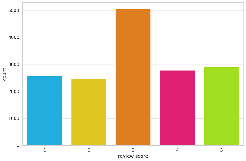

That’s hugely imbalanced, but it’s okay. We’re going to convert the dataset into negative, neutral and positive sentiment:

1def to_sentiment(rating):
2  rating = int(rating)
3  if rating <= 2:
4    return 0
5  elif rating == 3:
6    return 1
7  else:
8    return 2
9
10df['sentiment'] = df.score.apply(to_sentiment)

1class_names = ['negative', 'neutral', 'positive']

1ax = sns.countplot(df.sentiment)
2plt.xlabel('review sentiment')
3ax.set_xticklabels(class_names);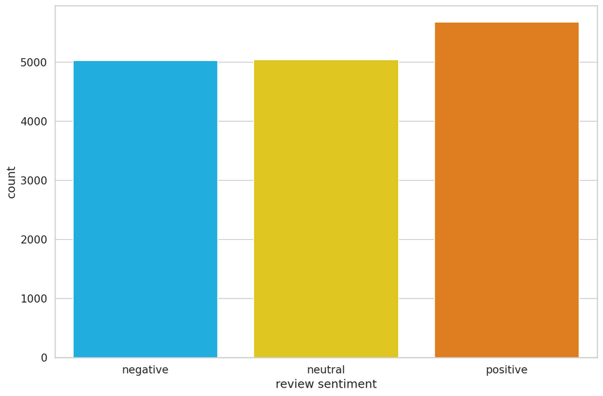

The balance was (mostly) restored.

Data Preprocessing

You might already know that Machine Learning models don’t work with raw text. You need to convert text to numbers (of some sort). BERT requires even more attention (good one, right?). Here are the requirements:

Add special tokens to separate sentences and do classification
Pass sequences of constant length (introduce padding)
Create array of 0s (pad token) and 1s (real token) called attention mask

The Transformers library provides (you’ve guessed it) a wide variety of Transformer models (including BERT). It works with TensorFlow and PyTorch! It also includes prebuild tokenizers that do the heavy lifting for us!

1PRE_TRAINED_MODEL_NAME = 'bert-base-cased'

You can use a cased and uncased version of BERT and tokenizer. I’ve experimented with both. The cased version works better. Intuitively, that makes sense, since “BAD” might convey more sentiment than “bad”.

Let’s load a pre-trained BertTokenizer:

1tokenizer = BertTokenizer.from_pretrained(PRE_TRAINED_MODEL_NAME)

We’ll use this text to understand the tokenization process:

1sample_txt = 'When was I last outside? I am stuck at home for 2 weeks.'

Some basic operations can convert the text to tokens and tokens to unique integers (ids):

1tokens = tokenizer.tokenize(sample_txt)
2token_ids = tokenizer.convert_tokens_to_ids(tokens)
3
4print(f' Sentence: {sample_txt}')
5print(f'   Tokens: {tokens}')
6print(f'Token IDs: {token_ids}')

1Sentence: When was I last outside? I am stuck at home for 2 weeks.
2   Tokens: ['When', 'was', 'I', 'last', 'outside', '?', 'I', 'am', 'stuck', 'at', 'home', 'for', '2', 'weeks', '.']
3Token IDs: [1332, 1108, 146, 1314, 1796, 136, 146, 1821, 5342, 1120, 1313, 1111, 123, 2277, 119]

Special Tokens

[SEP] - marker for ending of a sentence

1tokenizer.sep_token, tokenizer.sep_token_id

1('[SEP]', 102)

[CLS] - we must add this token to the start of each sentence, so BERT knows we’re doing classification

1tokenizer.cls_token, tokenizer.cls_token_id

1('[CLS]', 101)

There is also a special token for padding:

1tokenizer.pad_token, tokenizer.pad_token_id

1('[PAD]', 0)

BERT understands tokens that were in the training set. Everything else can be encoded using the [UNK] (unknown) token:

1tokenizer.unk_token, tokenizer.unk_token_id

1('[UNK]', 100)

All of that work can be done using the encode_plus() method:

1encoding = tokenizer.encode_plus(
2  sample_txt,
3  max_length=32,
4  add_special_tokens=True, # Add '[CLS]' and '[SEP]'
5  return_token_type_ids=False,
6  pad_to_max_length=True,
7  return_attention_mask=True,
8  return_tensors='pt',  # Return PyTorch tensors
9)
10
11encoding.keys()

1dict_keys(['input_ids', 'attention_mask'])

The token ids are now stored in a Tensor and padded to a length of 32:

1print(len(encoding['input_ids'][0]))
2encoding['input_ids'][0]

132
2tensor([ 101, 1332, 1108,  146, 1314, 1796,  136,  146, 1821, 5342, 1120, 1313,
3        1111,  123, 2277,  119,  102,    0,    0,    0,    0,    0,    0,    0,
4           0,    0,    0,    0,    0,    0,    0,    0])

The attention mask has the same length:

1print(len(encoding['attention_mask'][0]))
2encoding['attention_mask']

132
2tensor([[1, 1, 1, 1, 1, 1, 1, 1, 1, 1, 1, 1, 1, 1, 1, 1, 1, 0, 0, 0, 0, 0, 0, 0,
3         0, 0, 0, 0, 0, 0, 0, 0]])

We can inverse the tokenization to have a look at the special tokens:

1tokenizer.convert_ids_to_tokens(encoding['input_ids'][0])

1['[CLS]',
2 'When',
3 'was',
4 'I',
5 'last',
6 'outside',
7 '?',
8 'I',
9 'am',
10 'stuck',
11 'at',
12 'home',
13 'for',
14 '2',
15 'weeks',
16 '.',
17 '[SEP]',
18 '[PAD]',
19 '[PAD]',
20 '[PAD]',
21 '[PAD]',
22 '[PAD]',
23 '[PAD]',
24 '[PAD]',
25 '[PAD]',
26 '[PAD]',
27 '[PAD]',
28 '[PAD]',
29 '[PAD]',
30 '[PAD]',
31 '[PAD]',
32 '[PAD]']

Choosing Sequence Length

BERT works with fixed-length sequences. We’ll use a simple strategy to choose the max length. Let’s store the token length of each review:

1token_lens = []
2
3for txt in df.content:
4  tokens = tokenizer.encode(txt, max_length=512)
5  token_lens.append(len(tokens))

and plot the distribution:

1sns.distplot(token_lens)
2plt.xlim([0, 256]);
3plt.xlabel('Token count');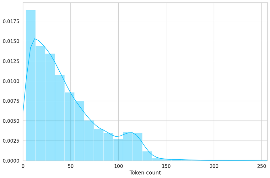

Most of the reviews seem to contain less than 128 tokens, but we’ll be on the safe side and choose a maximum length of 160.

1MAX_LEN = 160

We have all building blocks required to create a PyTorch dataset. Let’s do it:

1class GPReviewDataset(Dataset):
2
3  def __init__(self, reviews, targets, tokenizer, max_len):
4    self.reviews = reviews
5    self.targets = targets
6    self.tokenizer = tokenizer
7    self.max_len = max_len
8
9  def __len__(self):
10    return len(self.reviews)
11
12  def __getitem__(self, item):
13    review = str(self.reviews[item])
14    target = self.targets[item]
15
16    encoding = self.tokenizer.encode_plus(
17      review,
18      add_special_tokens=True,
19      max_length=self.max_len,
20      return_token_type_ids=False,
21      pad_to_max_length=True,
22      return_attention_mask=True,
23      return_tensors='pt',
24    )
25
26    return {
27      'review_text': review,
28      'input_ids': encoding['input_ids'].flatten(),
29      'attention_mask': encoding['attention_mask'].flatten(),
30      'targets': torch.tensor(target, dtype=torch.long)
31    }

The tokenizer is doing most of the heavy lifting for us. We also return the review texts, so it’ll be easier to evaluate the predictions from our model. Let’s split the data:

1df_train, df_test = train_test_split(
2  df,
3  test_size=0.1,
4  random_state=RANDOM_SEED
5)
6df_val, df_test = train_test_split(
7  df_test,
8  test_size=0.5,
9  random_state=RANDOM_SEED
10)

1df_train.shape, df_val.shape, df_test.shape

1((14171, 12), (787, 12), (788, 12))

We also need to create a couple of data loaders. Here’s a helper function to do it:

1def create_data_loader(df, tokenizer, max_len, batch_size):
2  ds = GPReviewDataset(
3    reviews=df.content.to_numpy(),
4    targets=df.sentiment.to_numpy(),
5    tokenizer=tokenizer,
6    max_len=max_len
7  )
8
9  return DataLoader(
10    ds,
11    batch_size=batch_size,
12    num_workers=4
13  )

1BATCH_SIZE = 16
2
3train_data_loader = create_data_loader(df_train, tokenizer, MAX_LEN, BATCH_SIZE)
4val_data_loader = create_data_loader(df_val, tokenizer, MAX_LEN, BATCH_SIZE)
5test_data_loader = create_data_loader(df_test, tokenizer, MAX_LEN, BATCH_SIZE)

Let’s have a look at an example batch from our training data loader:

1data = next(iter(train_data_loader))
2data.keys()

1dict_keys(['review_text', 'input_ids', 'attention_mask', 'targets'])

1print(data['input_ids'].shape)
2print(data['attention_mask'].shape)
3print(data['targets'].shape)

1torch.Size([16, 160])
2torch.Size([16, 160])
3torch.Size([16])

Sentiment Classification with BERT and Hugging Face

There are a lot of helpers that make using BERT easy with the Transformers library. Depending on the task you might want to use BertForSequenceClassification, BertForQuestionAnswering or something else.

But who cares, right? We’re hardcore! We’ll use the basic BertModel and build our sentiment classifier on top of it. Let’s load the model:

1bert_model = BertModel.from_pretrained(PRE_TRAINED_MODEL_NAME)

And try to use it on the encoding of our sample text:

1last_hidden_state, pooled_output = bert_model(
2  input_ids=encoding['input_ids'],
3  attention_mask=encoding['attention_mask']
4)

The last_hidden_state is a sequence of hidden states of the last layer of the model. Obtaining the pooled_output is done by applying the BertPooler on last_hidden_state:

1last_hidden_state.shape

1torch.Size([1, 32, 768])

We have the hidden state for each of our 32 tokens (the length of our example sequence). But why 768? This is the number of hidden units in the feedforward-networks. We can verify that by checking the config:

1bert_model.config.hidden_size

You can think of the pooled_output as a summary of the content, according to BERT. Albeit, you might try and do better. Let’s look at the shape of the output:

1pooled_output.shape

1torch.Size([1, 768])

We can use all of this knowledge to create a classifier that uses the BERT model:

1class SentimentClassifier(nn.Module):
2
3  def __init__(self, n_classes):
4    super(SentimentClassifier, self).__init__()
5    self.bert = BertModel.from_pretrained(PRE_TRAINED_MODEL_NAME)
6    self.drop = nn.Dropout(p=0.3)
7    self.out = nn.Linear(self.bert.config.hidden_size, n_classes)
8
9  def forward(self, input_ids, attention_mask):
10    _, pooled_output = self.bert(
11      input_ids=input_ids,
12      attention_mask=attention_mask
13    )
14    output = self.drop(pooled_output)
15    return self.out(output

Our classifier delegates most of the heavy lifting to the BertModel. We use a dropout layer for some regularization and a fully-connected layer for our output. Note that we’re returning the raw output of the last layer since that is required for the cross-entropy loss function in PyTorch to work.

This should work like any other PyTorch model. Let’s create an instance and move it to the GPU

1model = SentimentClassifier(len(class_names))
2model = model.to(device)

We’ll move the example batch of our training data to the GPU:

1input_ids = data['input_ids'].to(device)
2attention_mask = data['attention_mask'].to(device)
3
4print(input_ids.shape) # batch size x seq length
5print(attention_mask.shape) # batch size x seq length

1torch.Size([16, 160])
2torch.Size([16, 160])

To get the predicted probabilities from our trained model, we’ll apply the softmax function to the outputs:

1F.softmax(model(input_ids, attention_mask), dim=1)

1tensor([[0.5879, 0.0842, 0.3279],
2        [0.4308, 0.1888, 0.3804],
3        [0.4871, 0.1766, 0.3363],
4        [0.3364, 0.0778, 0.5858],
5        [0.4025, 0.1040, 0.4935],
6        [0.3599, 0.1026, 0.5374],
7        [0.5054, 0.1552, 0.3394],
8        [0.5962, 0.1464, 0.2574],
9        [0.3274, 0.1967, 0.4759],
10        [0.3026, 0.1118, 0.5856],
11        [0.4103, 0.1571, 0.4326],
12        [0.4879, 0.2121, 0.3000],
13        [0.3811, 0.1477, 0.4712],
14        [0.3354, 0.1354, 0.5292],
15        [0.3999, 0.2822, 0.3179],
16        [0.5075, 0.1684, 0.3242]], device='cuda:0', grad_fn=<SoftmaxBackward>)

Training

To reproduce the training procedure from the BERT paper, we’ll use the AdamW optimizer provided by Hugging Face. It corrects weight decay, so it’s similar to the original paper. We’ll also use a linear scheduler with no warmup steps:

1EPOCHS = 10
2
3optimizer = AdamW(model.parameters(), lr=2e-5, correct_bias=False)
4total_steps = len(train_data_loader) * EPOCHS
5
6scheduler = get_linear_schedule_with_warmup(
7  optimizer,
8  num_warmup_steps=0,
9  num_training_steps=total_steps
10)
11
12loss_fn = nn.CrossEntropyLoss().to(device)

How do we come up with all hyperparameters? The BERT authors have some recommendations for fine-tuning:

Batch size: 16, 32
Learning rate (Adam): 5e-5, 3e-5, 2e-5
Number of epochs: 2, 3, 4

We’re going to ignore the number of epochs recommendation but stick with the rest. Note that increasing the batch size reduces the training time significantly, but gives you lower accuracy.

Let’s continue with writing a helper function for training our model for one epoch:

1def train_epoch(
2  model,
3  data_loader,
4  loss_fn,
5  optimizer,
6  device,
7  scheduler,
8  n_examples
9):
10  model = model.train()
11
12  losses = []
13  correct_predictions = 0
14
15  for d in data_loader:
16    input_ids = d["input_ids"].to(device)
17    attention_mask = d["attention_mask"].to(device)
18    targets = d["targets"].to(device)
19
20    outputs = model(
21      input_ids=input_ids,
22      attention_mask=attention_mask
23    )
24
25    _, preds = torch.max(outputs, dim=1)
26    loss = loss_fn(outputs, targets)
27
28    correct_predictions += torch.sum(preds == targets)
29    losses.append(loss.item())
30
31    loss.backward()
32    nn.utils.clip_grad_norm_(model.parameters(), max_norm=1.0)
33    optimizer.step()
34    scheduler.step()
35    optimizer.zero_grad()
36
37  return correct_predictions.double() / n_examples, np.mean(losses)

Training the model should look familiar, except for two things. The scheduler gets called every time a batch is fed to the model. We’re avoiding exploding gradients by clipping the gradients of the model using clipgrad_norm.

Let’s write another one that helps us evaluate the model on a given data loader:

1def eval_model(model, data_loader, loss_fn, device, n_examples):
2  model = model.eval()
3
4  losses = []
5  correct_predictions = 0
6
7  with torch.no_grad():
8    for d in data_loader:
9      input_ids = d["input_ids"].to(device)
10      attention_mask = d["attention_mask"].to(device)
11      targets = d["targets"].to(device)
12
13      outputs = model(
14        input_ids=input_ids,
15        attention_mask=attention_mask
16      )
17      _, preds = torch.max(outputs, dim=1)
18
19      loss = loss_fn(outputs, targets)
20
21      correct_predictions += torch.sum(preds == targets)
22      losses.append(loss.item())
23
24  return correct_predictions.double() / n_examples, np.mean(losses)

Using those two, we can write our training loop. We’ll also store the training history:

1%%time
2
3history = defaultdict(list)
4best_accuracy = 0
5
6for epoch in range(EPOCHS):
7
8  print(f'Epoch {epoch + 1}/{EPOCHS}')
9  print('-' * 10)
10
11  train_acc, train_loss = train_epoch(
12    model,
13    train_data_loader,
14    loss_fn,
15    optimizer,
16    device,
17    scheduler,
18    len(df_train)
19  )
20
21  print(f'Train loss {train_loss} accuracy {train_acc}')
22
23  val_acc, val_loss = eval_model(
24    model,
25    val_data_loader,
26    loss_fn,
27    device,
28    len(df_val)
29  )
30
31  print(f'Val   loss {val_loss} accuracy {val_acc}')
32  print()
33
34  history['train_acc'].append(train_acc)
35  history['train_loss'].append(train_loss)
36  history['val_acc'].append(val_acc)
37  history['val_loss'].append(val_loss)
38
39  if val_acc > best_accuracy:
40    torch.save(model.state_dict(), 'best_model_state.bin')
41    best_accuracy = val_acc

1Epoch 1/10
2----------
3Train loss 0.7330631300571541 accuracy 0.6653729447463129
4Val   loss 0.5767546480894089 accuracy 0.7776365946632783
5
6Epoch 2/10
7----------
8Train loss 0.4158683338330777 accuracy 0.8420012701997036
9Val   loss 0.5365073362737894 accuracy 0.832274459974587
10
11Epoch 3/10
12----------
13Train loss 0.24015077009679367 accuracy 0.922023851527768
14Val   loss 0.5074492372572422 accuracy 0.8716645489199493
15
16Epoch 4/10
17----------
18Train loss 0.16012676668187295 accuracy 0.9546962105708843
19Val   loss 0.6009970247745514 accuracy 0.8703939008894537
20
21Epoch 5/10
22----------
23Train loss 0.11209654617575301 accuracy 0.9675393409074872
24Val   loss 0.7367783848941326 accuracy 0.8742058449809403
25
26Epoch 6/10
27----------
28Train loss 0.08572274737026433 accuracy 0.9764307388328276
29Val   loss 0.7251267762482166 accuracy 0.8843710292249047
30
31Epoch 7/10
32----------
33Train loss 0.06132202987342602 accuracy 0.9833462705525369
34Val   loss 0.7083295831084251 accuracy 0.889453621346887
35
36Epoch 8/10
37----------
38Train loss 0.050604159273123096 accuracy 0.9849693035071626
39Val   loss 0.753860274553299 accuracy 0.8907242693773825
40
41Epoch 9/10
42----------
43Train loss 0.04373276197092931 accuracy 0.9862395032107826
44Val   loss 0.7506809896230697 accuracy 0.8919949174078781
45
46Epoch 10/10
47----------
48Train loss 0.03768671146314381 accuracy 0.9880036694658105
49Val   loss 0.7431786182522774 accuracy 0.8932655654383737
50
51CPU times: user 29min 54s, sys: 13min 28s, total: 43min 23s
52Wall time: 43min 43s

Note that we’re storing the state of the best model, indicated by the highest validation accuracy.

Whoo, this took some time! We can look at the training vs validation accuracy:

1plt.plot(history['train_acc'], label='train accuracy')
2plt.plot(history['val_acc'], label='validation accuracy')
3
4plt.title('Training history')
5plt.ylabel('Accuracy')
6plt.xlabel('Epoch')
7plt.legend()
8plt.ylim([0, 1]);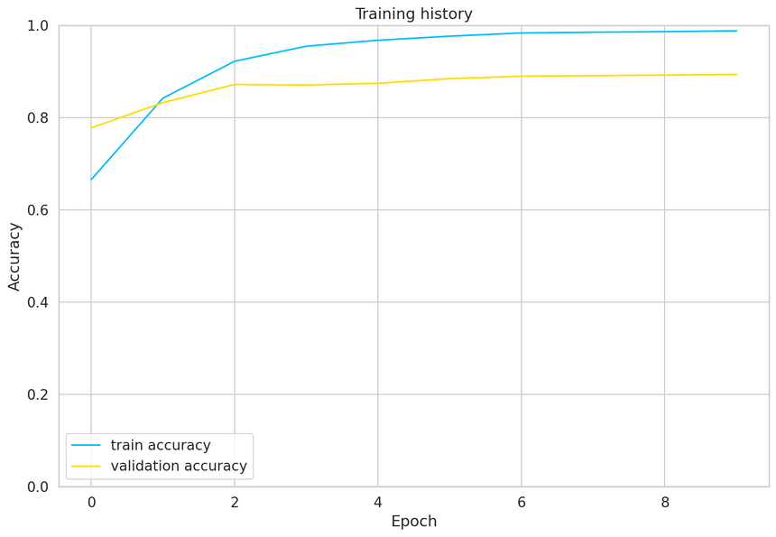

The training accuracy starts to approach 100% after 10 epochs or so. You might try to fine-tune the parameters a bit more, but this will be good enough for us.

Don’t want to wait? Uncomment the next cell to download my pre-trained model:

1# !gdown --id 1V8itWtowCYnb2Bc9KlK9SxGff9WwmogA
2
3# model = SentimentClassifier(len(class_names))
4# model.load_state_dict(torch.load('best_model_state.bin'))
5# model = model.to(device)

Evaluation

So how good is our model on predicting sentiment? Let’s start by calculating the accuracy on the test data:

1test_acc, _ = eval_model(
2  model,
3  test_data_loader,
4  loss_fn,
5  device,
6  len(df_test)
7)
8
9test_acc.item()

10.883248730964467

The accuracy is about 1% lower on the test set. Our model seems to generalize well.

We’ll define a helper function to get the predictions from our model:

1def get_predictions(model, data_loader):
2  model = model.eval()
3
4  review_texts = []
5  predictions = []
6  prediction_probs = []
7  real_values = []
8
9  with torch.no_grad():
10    for d in data_loader:
11
12      texts = d["review_text"]
13      input_ids = d["input_ids"].to(device)
14      attention_mask = d["attention_mask"].to(device)
15      targets = d["targets"].to(device)
16
17      outputs = model(
18        input_ids=input_ids,
19        attention_mask=attention_mask
20      )
21      _, preds = torch.max(outputs, dim=1)
22
23      review_texts.extend(texts)
24      predictions.extend(preds)
25      prediction_probs.extend(outputs)
26      real_values.extend(targets)
27
28  predictions = torch.stack(predictions).cpu()
29  prediction_probs = torch.stack(prediction_probs).cpu()
30  real_values = torch.stack(real_values).cpu()
31  return review_texts, predictions, prediction_probs, real_values

This is similar to the evaluation function, except that we’re storing the text of the reviews and the predicted probabilities:

1y_review_texts, y_pred, y_pred_probs, y_test = get_predictions(
2  model,
3  test_data_loader
4)

Let’s have a look at the classification report

1print(classification_report(y_test, y_pred, target_names=class_names))

1precision    recall  f1-score   support
2
3    negative       0.89      0.87      0.88       245
4     neutral       0.83      0.85      0.84       254
5    positive       0.92      0.93      0.92       289
6
7    accuracy                           0.88       788
8   macro avg       0.88      0.88      0.88       788
9weighted avg       0.88      0.88      0.88       788

Looks like it is really hard to classify neutral (3 stars) reviews. And I can tell you from experience, looking at many reviews, those are hard to classify.

We’ll continue with the confusion matrix:

1def show_confusion_matrix(confusion_matrix):
2  hmap = sns.heatmap(confusion_matrix, annot=True, fmt="d", cmap="Blues")
3  hmap.yaxis.set_ticklabels(hmap.yaxis.get_ticklabels(), rotation=0, ha='right')
4  hmap.xaxis.set_ticklabels(hmap.xaxis.get_ticklabels(), rotation=30, ha='right')
5  plt.ylabel('True sentiment')
6  plt.xlabel('Predicted sentiment');
7
8cm = confusion_matrix(y_test, y_pred)
9df_cm = pd.DataFrame(cm, index=class_names, columns=class_names)
10show_confusion_matrix(df_cm)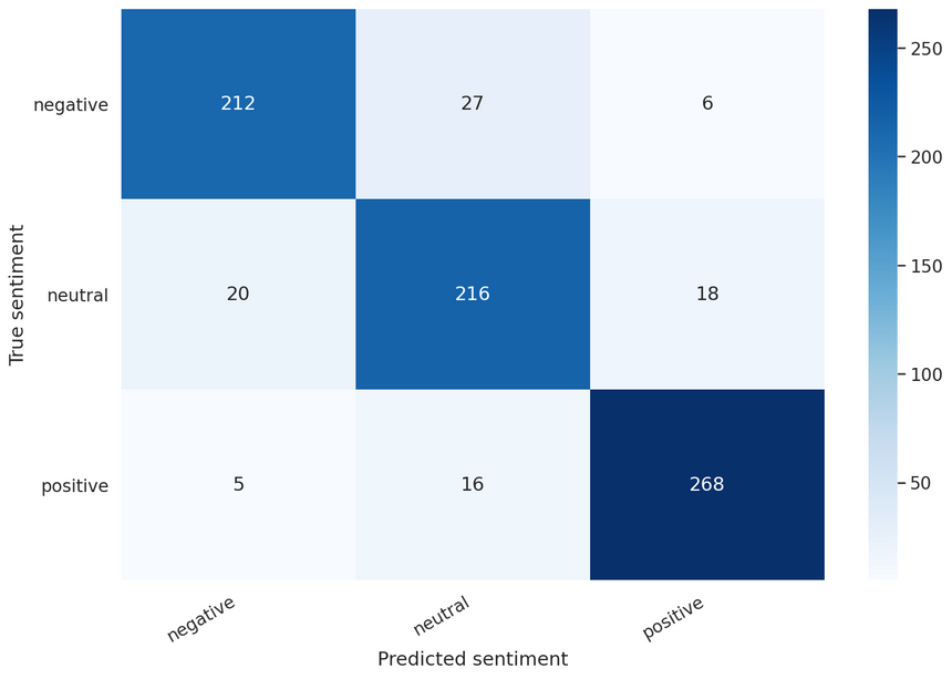

This confirms that our model is having difficulty classifying neutral reviews. It mistakes those for negative and positive at a roughly equal frequency.

That’s a good overview of the performance of our model. But let’s have a look at an example from our test data:

1idx = 2
2
3review_text = y_review_texts[idx]
4true_sentiment = y_test[idx]
5pred_df = pd.DataFrame({
6  'class_names': class_names,
7  'values': y_pred_probs[idx]
8})

1print("\n".join(wrap(review_text)))
2print()
3print(f'True sentiment: {class_names[true_sentiment]}')

1I used to use Habitica, and I must say this is a great step up. I'd
2like to see more social features, such as sharing tasks - only one
3person has to perform said task for it to be checked off, but only
4giving that person the experience and gold. Otherwise, the price for
5subscription is too steep, thus resulting in a sub-perfect score. I
6could easily justify $0.99/month or eternal subscription for $15. If
7that price could be met, as well as fine tuning, this would be easily
8worth 5 stars.
9
10True sentiment: neutral

Now we can look at the confidence of each sentiment of our model:

1sns.barplot(x='values', y='class_names', data=pred_df, orient='h')
2plt.ylabel('sentiment')
3plt.xlabel('probability')
4plt.xlim([0, 1]);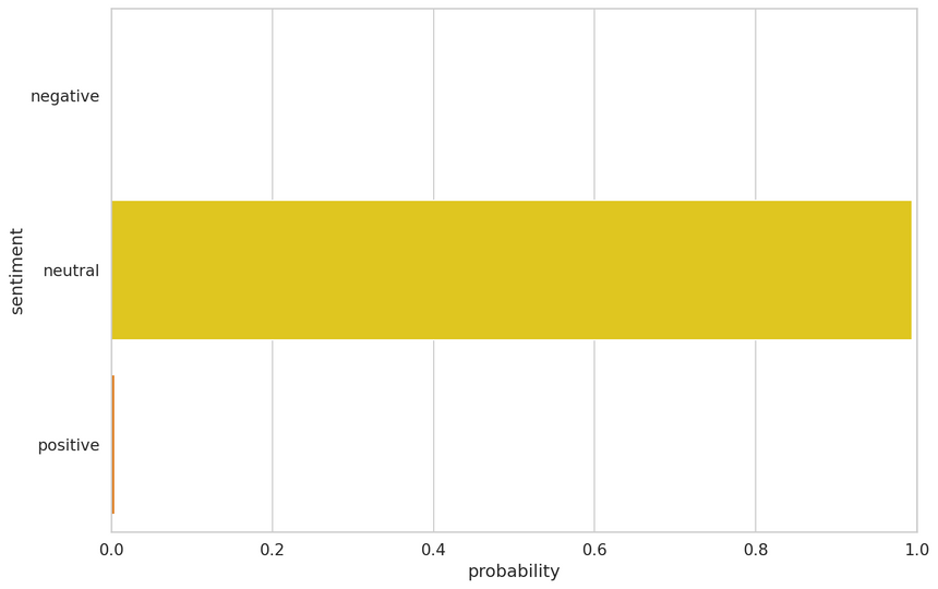

Predicting on Raw Text

Let’s use our model to predict the sentiment of some raw text:

1review_text = "I love completing my todos! Best app ever!!!"

We have to use the tokenizer to encode the text:

1encoded_review = tokenizer.encode_plus(
2  review_text,
3  max_length=MAX_LEN,
4  add_special_tokens=True,
5  return_token_type_ids=False,
6  pad_to_max_length=True,
7  return_attention_mask=True,
8  return_tensors='pt',
9)

Let’s get the predictions from our model:

1input_ids = encoded_review['input_ids'].to(device)
2attention_mask = encoded_review['attention_mask'].to(device)
3
4output = model(input_ids, attention_mask)
5_, prediction = torch.max(output, dim=1)
6
7print(f'Review text: {review_text}')
8print(f'Sentiment  : {class_names[prediction]}')

1Review text: I love completing my todos! Best app ever!!!
2Sentiment  : positive

Summary

Nice job! You learned how to use BERT for sentiment analysis. You built a custom classifier using the Hugging Face library and trained it on our app reviews dataset!

You learned how to:

Intuitively understand what BERT is
Preprocess text data for BERT and build PyTorch Dataset (tokenization, attention masks, and padding)
Use Transfer Learning to build Sentiment Classifier using the Transformers library by Hugging Face
Evaluate the model on test data
Predict sentiment on raw text

Next, we’ll learn how to deploy our trained model behind a REST API and build a simple web app to access it.

References

Want to be a Machine Learning expert?

Join the weekly newsletter on Data Science, Deep Learning and Machine Learning in your inbox, curated by me! Chosen by 10,000+ Machine Learning practitioners. (There might be some exclusive content, too!)

You'll never get spam from me

Hacker's Guide to Neural Networks in JavaScript

Build Machine Learning models (especially Deep Neural Networks) that you can easily integrate with existing or new web apps. Think of your ReactJs, Vue, or Angular app enhanced with the power of Machine Learning models.

Get SH*T Done with PyTorch

Learn how to solve real-world problems with Deep Learning models (NLP, Computer Vision, and Time Series). Go from prototyping to deployment with PyTorch and Python!

Hacker's Guide to Machine Learning with Python

This book brings the fundamentals of Machine Learning to you, using tools and techniques used to solve real-world problems in Computer Vision, Natural Language Processing, and Time Series analysis. The skills taught in this book will lay the foundation for you to advance your journey to Machine Learning Mastery!

Hands-On Machine Learning from Scratch

This book will guide you on your journey to deeper Machine Learning understanding by developing algorithms in Python from scratch! Learn why and when Machine learning is the right tool for the job and how to improve low performing models!