TL;DR Learn how to use Tensors, build a Linear Regression model and a simple Neural Network

TensorFlow 2.0 (final) was released at the end of September. Oh boy, it looks much cooler than the 1.x series. Why is it so much better for you, the developer?

• One high-level API for building models (that you know and love) - Keras. The good news is that most of your old Keras code should work automagically after changing a couple of imports.

• Eager execution - all your code looks much more like normal Python programs. Old-timers might remember the horrible Session experiences. You shouldn’t need any of that, in day-to-day use.

There are tons of other improvements, but the new developer experience is something that will make using TensorFlow 2 sweeter. What about PyTorch? PyTorch is still great and easy to use. But it seems like TensorFlow is catching up, or is it?

You’ll learn:

• How to install TensorFlow 2
• What is a Tensor
• Doing Tensor math
• Using probability distributions and sampling
• Build a Simple Linear Regression model
• Build a Simple Neural Network model
• Save/restore a model

Run the complete code in your browser

Setup

Let’s install the GPU-supported version and set up the environment:

1!pip install tensorflow-gpu

Check the installed version:

1import tensorflow as tf
2
3tf.__version__

12.0.0

And specify a random seed, so our results are reproducible:

1RANDOM_SEED = 42
2
3tf.random.set_seed(RANDOM_SEED)

Tensors

TensorFlow allows you to define and run operations on Tensors. Tensors are data-containers that can be of arbitrary dimension - scalars, vectors, matrices, etc. You can put numbers (floats and ints) and strings into Tensors.

Let’s create a simple Tensor:

1x = tf.constant(1)
2print(x)

1tf.Tensor(1, shape=(), dtype=int32)

It seems like our first Tensor contains the number 1, it is of type int32 and is shapeless. To obtain the value we can do:

1x.numpy()

11

Let’s create a simple matrix:

1m = tf.constant([[1, 2, 1], [3, 4, 2]])
2print(m)

1tf.Tensor(
2[[1 2 1]
3 [3 4 2]], shape=(2, 3), dtype=int32)

This shape thingy seems to specify rows x columns. In general, the shape array shows how many elements are in every dimension of the Tensor.

Helpers

TensorFlow offers a variety of helper functions for creating Tensors. Let’s create a matrix full of ones:

1ones = tf.ones([3, 3])
2print(ones)

1tf.Tensor(
2[[1. 1. 1.]
3 [1. 1. 1.]
4 [1. 1. 1.]], shape=(3, 3), dtype=float32)

and zeros:

1zeros = tf.zeros([2, 3])
2print(zeros)

1tf.Tensor(
2[[0. 0. 0.]
3 [0. 0. 0.]], shape=(2, 3), dtype=float32)

We have two rows and three columns. What if we want to turn it into three rows and two columns:

1tf.reshape(zeros, [3, 2])

1tf.Tensor(
2[[0. 0.]
3 [0. 0.]
4 [0. 0.]], shape=(3, 2), dtype=float32)

You can use another helper function to replace rows and columns (transpose):

1tf.transpose(zeros)

1tf.Tensor(
2[[0. 0.]
3 [0. 0.]
4 [0. 0.]], shape=(3, 2), dtype=float32)

Tensor Math

Naturally, you would want to do something with your data. Let’s start with adding numbers:

1a = tf.constant(1)
2b = tf.constant(1)
3
4tf.add(a, b).numpy()

142

That seems reasonable :) You can do the same thing using something more human friendly:

1(a + b).numpy()

You can multiply Tensors like so:

1c = a + b
2c * c

And compute dot product of matrices:

1d1 = tf.constant([[1, 2], [1, 2]]);
2d2 = tf.constant([[3, 4], [3, 4]]);
3
4tf.tensordot(d1, d2, axes=1).numpy()

1array([[ 9, 12],
2       [ 9, 12]], dtype=int32)

Sampling

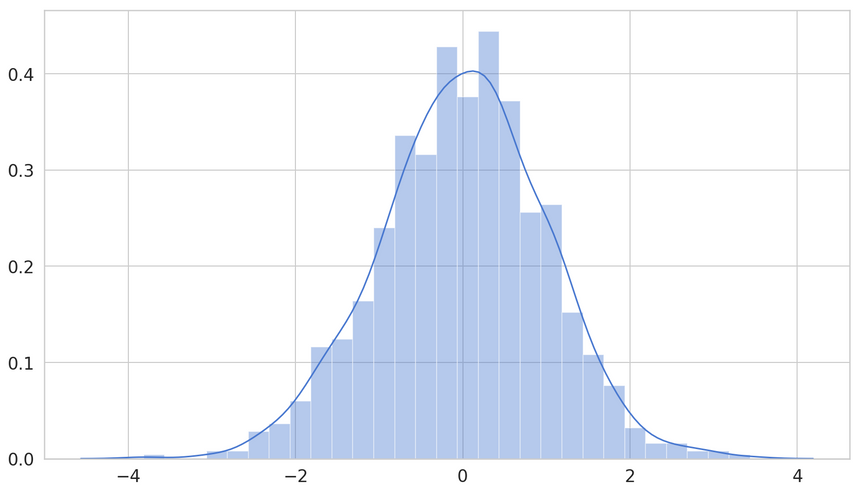
You can also generate random numbers according to some famous probability distributions. Let’s start with Normal:

1norm = tf.random.normal(shape=(1000, 1), mean=0., stddev=1.)

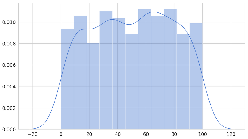
We can do the same thing from the Uniform:

1unif = tf.random.uniform(shape=(1000, 1), minval=0, maxval=100)

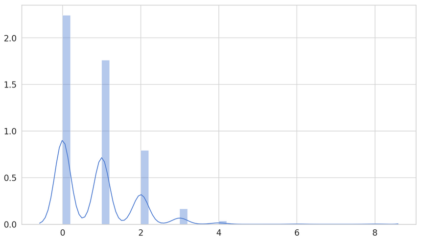
Let’s have a look at something a tad more exotic - the Poisson distribution. It is popular for modeling the number of times an event occurs in some time. It is the first one (in our exploration) that contains a hyperparameter - $\lambda$. It controls the number of expected occurrences.

1pois = tf.random.poisson(shape=(1000, 1), lam=0.8)

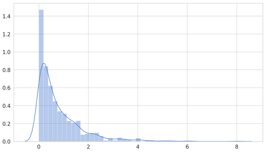
The Gamma distribution is continuous. It has 2 hyperparameters that control the shape and scale. It is used to model always positive continuous variables with skewed distributions.

1gam = tf.random.gamma(shape=(1000, 1), alpha=0.8)

Simple Linear Regression Model

Let’s build a Simple Linear Regression model to predict the stopping distance of cars based on their speed. The data comes from here: https://vincentarelbundock.github.io/Rdatasets/datasets.html. It is given by this Tensor:

1data = tf.constant([
2  [4,2],
3  [4,10],
4  [7,4],
5  [7,22],
6  [8,16],
7  [9,10],
8  [10,18],
9  [10,26],
10  [10,34],
11  [11,17],
12  [11,28],
13  [12,14],
14  [12,20],
15  [12,24],
16  [12,28],
17  [13,26],
18  [13,34],
19  [13,34],
20  [13,46],
21  [14,26],
22  [14,36],
23  [14,60],
24  [14,80],
25  [15,20],
26  [15,26],
27  [15,54],
28  [16,32],
29  [16,40],
30  [17,32],
31  [17,40],
32  [17,50],
33  [18,42],
34  [18,56],
35  [18,76],
36  [18,84],
37  [19,36],
38  [19,46],
39  [19,68],
40  [20,32],
41  [20,48],
42  [20,52],
43  [20,56],
44  [20,64],
45  [22,66],
46  [23,54],
47  [24,70],
48  [24,92],
49  [24,93],
50  [24,120],
51  [25,85]
52])

We can extract the two columns using slicing:

1speed = data[:, 0]
2stopping_distance = data[:, 1]

Let’s have a look at the data:

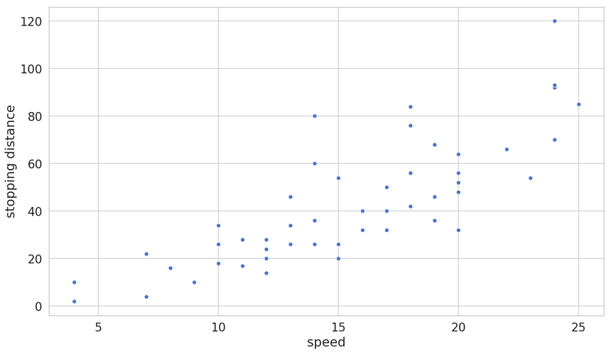
It seems like a linear model can do a decent job of predicting the stopping distance. Simple Linear Regression finds a straight line that predicts the variable of interest based on a single predictor/feature.

Time to build the model using the Keras API:

1lin_reg = keras.Sequential([
2  layers.Dense(1, activation='linear', input_shape=[1]),
3])
4
5optimizer = tf.keras.optimizers.RMSprop(0.001)
6
7lin_reg.compile(
8  loss='mse',
9  optimizer=optimizer,
10  metrics=['mse']
11)

We’re using the Sequential API with a single layer - 1 parameter with linear activation. We’ll try to minimize the Mean squared error during training.

And for the training itself:

1history = lin_reg.fit(
2  x=speed,
3  y=stopping_distance,
4  shuffle=True,
5  epochs=1000,
6  validation_split=0.2,
7  verbose=0
8)

We’re breaking any ordering issues by shuffling the data and reserving 20% for validation. Let’s have a look at the training process:

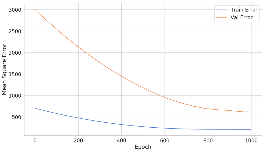
The model is steadily improving during training. That’s a good sign. What can we do with a more complex model?

Simple Neural Network Model

Keras (and TensorFlow) was designed as a tool to build Neural Networks. Turns out, Neural Networks are good when a linear model isn’t enough. Let’s create one:

1def build_neural_net():
2  net = keras.Sequential([
3    layers.Dense(32, activation='relu', input_shape=[1]),
4    layers.Dense(16, activation='relu'),
5    layers.Dense(1),
6  ])
7
8  optimizer = tf.keras.optimizers.RMSprop(0.001)
9
10  net.compile(loss='mse',
11                optimizer=optimizer,
12                metrics=['mse', 'accuracy'])
13
14  return net

Things look similar, except for the fact that we stack multiple layers on top of each other. We’re also using a different activation function - ReLU.

Training this model looks exactly the same:

1net = build_neural_net()
2
3history = net.fit(
4  x=speed,
5  y=stopping_distance,
6  shuffle=True,
7  epochs=1000,
8  validation_split=0.2,
9  verbose=0
10)

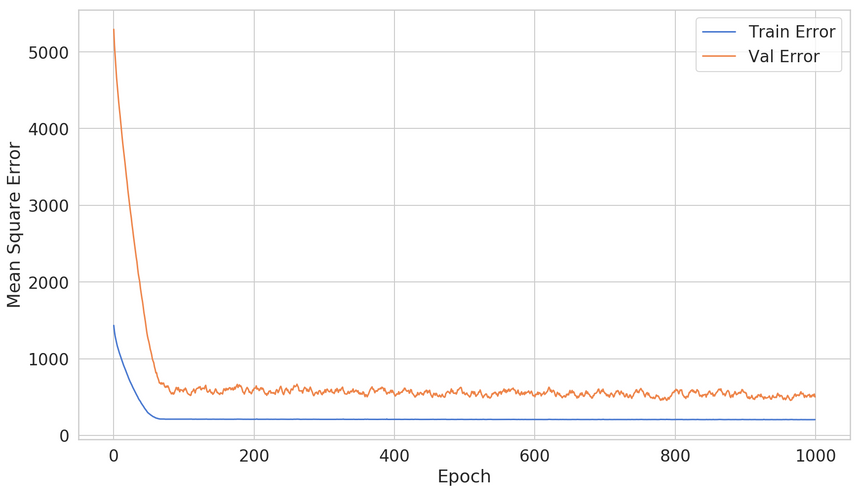
Seems like we ain’t making much progress after epoch 200 or so. Can we not waste our time waiting for the whole training to complete?

Early Stopping

Sure, you can stop the training process manually at say epoch 200. But what if you train another model? What if you obtain more data?

You can use the built-in callback EarlyStopping to halt the training when some metric (e.g. the validation loss) stops improving. Let’s see how we can use it:

1early_stop = keras.callbacks.EarlyStopping(
2  monitor='val_loss',
3  patience=10
4)

We want to monitor the validation loss. We’ll observe for improvement for 10 epochs before stopping. Let’s see how we can use it:

1net = build_neural_net()
2
3history = net.fit(
4  x=speed,
5  y=stopping_distance,
6  shuffle=True,
7  epochs=1000,
8  validation_split=0.2,
9  verbose=0,
10  callbacks=[early_stop]
11)

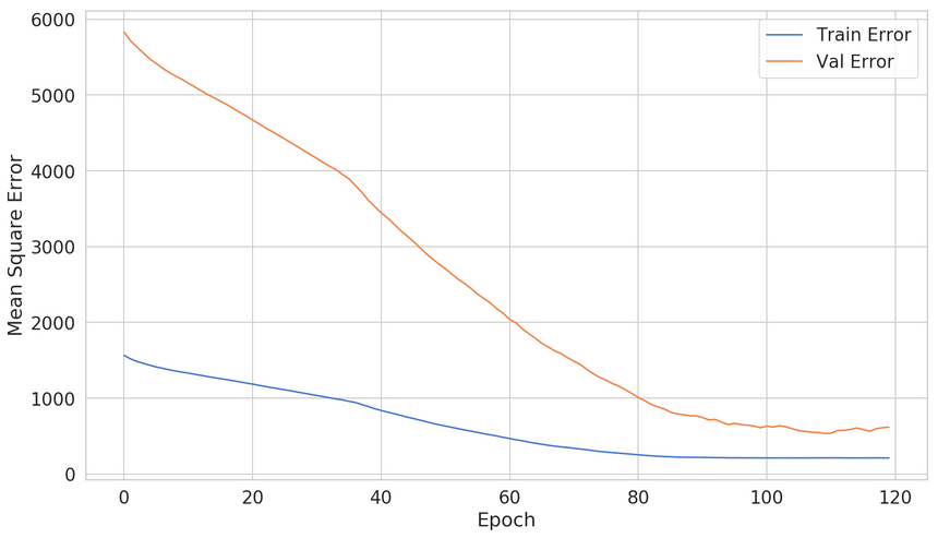
Effectively, we’ve cut down the number of training epochs to ~120. Is this going to work every time that well? Not really. Using early stopping introduces yet another hyperparameter that you need to consider when training your model. Use it cautiously.

Now your model is ready for the real world. How can you store it for later use?

Save/Restore Model

You can save the complete model (including weights) like this:

1net.save('simple_net.h5')

And load it like that:

1simple_net = keras.models.load_model('simple_net.h5')

You can use this mechanism to deploy your model and use it in production (for example).

Conclusion

You did it! You now know (a tiny bit) TensorFlow 2! Let’s recap what you’ve learned:

• How to install TensorFlow 2
• What is a Tensor
• Doing Tensor math
• Using probability distributions and sampling
• Build a Simple Linear Regression model
• Build a Simple Neural Network model
• Save/restore a model

Run the complete code in your browser

Stay tuned for more :)

References

• TensorFlow 2.0 released

• TensorFlow 2.0 on GitHub

• Effective TensorFlow 2.0