Curiousily

Time Series Forecasting with LSTMs for Daily Coronavirus Cases using PyTorch in Python

05.03.2020 — Deep Learning, PyTorch, Machine Learning, Neural Network, Time Series, Python — 5 min read

TL;DR This tutorial is NOT trying to build a model that predicts the Covid-19 outbreak/pandemic in the best way possible. This is an example of how you can use Recurrent Neural Networks on some real-world Time Series data with PyTorch. Hopefully, there are much better models that predict the number of daily confirmed cases.

Time series data captures a series of data points recorded at (usually) regular intervals. Some common examples include daily weather temperature, stock prices, and the number of sales a company makes.

Many classical methods (e.g. ARIMA) try to deal with Time Series data with varying success (not to say they are bad at it). In the last couple of years, Long Short Term Memory Networks (LSTM) models have become a very useful method when dealing with those types of data.

Recurrent Neural Networks (LSTMs are one type of those) are very good at processing sequences of data. They can “recall” patterns in the data that are very far into the past (or future). In this tutorial, you’re going to learn how to use LSTMs to predict future Coronavirus cases based on real-world data.

Novel Coronavirus (COVID-19)

The novel Coronavirus (Covid-19) has spread around the world very rapidly. At the time of this writing, Worldometers.info shows that there are more than 95,488 confirmed cases in more than 84 countries.

The top 4 worst-affected (by far) are China (the source of the virus), South Korea, Italy, and Iran. Unfortunately, many cases are currently not reported due to:

A person can get infected without even knowing (asymptomatic)
Incorrect data reporting
Not enough test kits
The symptoms look a lot like the common flu

How dangerous is this virus?

Except for the common statistics you might see cited on the news, there are some good and some bad news:

More than 80% of the confirmed cases recover without any need of medical attention
3.4% Mortality Rate estimate by the World Health Organization (WHO) as of March 3
The reproductive number which represents the average number of people to which a single infected person will transmit the virus is between 1.4 and 2.5 (WHO’s estimated on Jan. 23)

The last one is really scary. It sounds like we can witness some crazy exponential growth if appropriate measures are not put in place.

Let’s get started!

1%reload_ext watermark
2%watermark -v -p numpy,pandas,torch

1CPython 3.6.9
2IPython 5.5.0
3
4numpy 1.17.5
5pandas 0.25.3
6torch 1.4.0

1import torch
2
3import os
4import numpy as np
5import pandas as pd
6from tqdm import tqdm
7import seaborn as sns
8from pylab import rcParams
9import matplotlib.pyplot as plt
10from matplotlib import rc
11from sklearn.preprocessing import MinMaxScaler
12from pandas.plotting import register_matplotlib_converters
13from torch import nn, optim
14
15%matplotlib inline
16%config InlineBackend.figure_format='retina'
17
18sns.set(style='whitegrid', palette='muted', font_scale=1.2)
19
20HAPPY_COLORS_PALETTE = ["#01BEFE", "#FFDD00", "#FF7D00", "#FF006D", "#93D30C", "#8F00FF"]
21
22sns.set_palette(sns.color_palette(HAPPY_COLORS_PALETTE))
23
24rcParams['figure.figsize'] = 14, 10
25register_matplotlib_converters()
26
27RANDOM_SEED = 42
28np.random.seed(RANDOM_SEED)
29torch.manual_seed(RANDOM_SEED)

Daily Cases Dataset

The data is provided by the Johns Hopkins University Center for Systems Science and Engineering (JHU CSSE) and contains the number of reported daily cases by country. The dataset is available on GitHub and is updated regularly.

We’re going to take the Time Series data only for confirmed cases (number of deaths and recovered cases are also available):

1# !wget https://raw.githubusercontent.com/CSSEGISandData/COVID-19/master/csse_covid_19_data/csse_covid_19_time_series/time_series_19-covid-Confirmed.csv

Or you can take the same dataset that I’ve used for this tutorial (the data snapshot is from 3 March 2020):

1!gdown --id 1AsfdLrGESCQnRW5rbMz56A1KBc3Fe5aV

Data exploration

Let’s load the data and have a peek:

1df = pd.read_csv('time_series_19-covid-Confirmed.csv')

Two things to note here:

The data contains a province, country, latitude, and longitude. We won’t be needing those.
The number of cases is cumulative. We’ll undo the accumulation.

Let’s start by getting rid of the first four columns:

1df = df.iloc[:, 4:]

Let’s check for missing values:

1df.isnull().sum().sum()

Everything seems to be in place. Let’s sum all rows, so we get the cumulative daily cases:

1daily_cases = df.sum(axis=0)
2daily_cases.index = pd.to_datetime(daily_cases.index)
3daily_cases.head()

12020-01-22     555
22020-01-23     653
32020-01-24     941
42020-01-25    1434
52020-01-26    2118
6dtype: int64

1plt.plot(daily_cases)
2plt.title("Cumulative daily cases");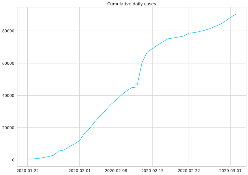

We’ll undo the accumulation by subtracting the current value from the previous. We’ll preserve the first value of the sequence:

1daily_cases = daily_cases.diff().fillna(daily_cases[0]).astype(np.int64)
2daily_cases.head()

12020-01-22    555
22020-01-23     98
32020-01-24    288
42020-01-25    493
52020-01-26    684
6dtype: int64

1plt.plot(daily_cases)
2plt.title("Daily cases");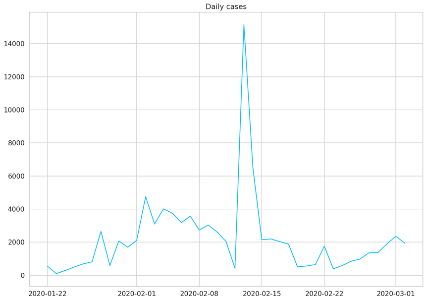

The huge spike (in the middle) is mostly due to a change of criteria for testing patients in China. This will certainly be a challenge for our model.

Let’s check the amount of data we have:

1daily_cases.shape

1(41,)

Unfortunately, we have data for only 41 days. Let’s see what we can do with it!

Preprocessing

We’ll reserve the first 27 days for training and use the rest for testing:

1test_data_size = 14
2
3train_data = daily_cases[:-test_data_size]
4test_data = daily_cases[-test_data_size:]
5
6train_data.shape

1(27,)

We have to scale the data (values will be between 0 and 1) if we want to increase the training speed and performance of the model. We’ll use the MinMaxScaler from scikit-learn:

1scaler = MinMaxScaler()
2
3scaler = scaler.fit(np.expand_dims(train_data, axis=1))
4
5train_data = scaler.transform(np.expand_dims(train_data, axis=1))
6
7test_data = scaler.transform(np.expand_dims(test_data, axis=1))

Currently, we have a big sequence of daily cases. We’ll convert it into smaller ones:

1def create_sequences(data, seq_length):
2    xs = []
3    ys = []
4
5    for i in range(len(data)-seq_length-1):
6        x = data[i:(i+seq_length)]
7        y = data[i+seq_length]
8        xs.append(x)
9        ys.append(y)
10
11    return np.array(xs), np.array(ys)

1seq_length = 5
2X_train, y_train = create_sequences(train_data, seq_length)
3X_test, y_test = create_sequences(test_data, seq_length)
4
5X_train = torch.from_numpy(X_train).float()
6y_train = torch.from_numpy(y_train).float()
7
8X_test = torch.from_numpy(X_test).float()
9y_test = torch.from_numpy(y_test).float()

Each training example contains a sequence of 5 data points of history and a label for the real value that our model needs to predict. Let’s dive in:

1X_train.shape

1torch.Size([21, 5, 1])

1X_train[:2]

1tensor([[[0.0304],
2         [0.0000],
3         [0.0126],
4         [0.0262],
5         [0.0389]],
6
7        [[0.0000],
8         [0.0126],
9         [0.0262],
10         [0.0389],
11         [0.0472]]])

1y_train.shape

1torch.Size([21, 1])

1y_train[:2]

1tensor([[0.0472],
2        [0.1696]])

1train_data[:10]

1array([[0.03036545],
2       [0.        ],
3       [0.01262458],
4       [0.02624585],
5       [0.03893688],
6       [0.04724252],
7       [0.16963455],
8       [0.03255814],
9       [0.13089701],
10       [0.10598007]])

Building a model

We’ll encapsulate the complexity of our model into a class that extends from torch.nn.Module:

1class CoronaVirusPredictor(nn.Module):
2
3  def __init__(self, n_features, n_hidden, seq_len, n_layers=2):
4    super(CoronaVirusPredictor, self).__init__()
5
6    self.n_hidden = n_hidden
7    self.seq_len = seq_len
8    self.n_layers = n_layers
9
10    self.lstm = nn.LSTM(
11      input_size=n_features,
12      hidden_size=n_hidden,
13      num_layers=n_layers,
14      dropout=0.5
15    )
16
17    self.linear = nn.Linear(in_features=n_hidden, out_features=1)
18
19  def reset_hidden_state(self):
20    self.hidden = (
21        torch.zeros(self.n_layers, self.seq_len, self.n_hidden),
22        torch.zeros(self.n_layers, self.seq_len, self.n_hidden)
23    )
24
25  def forward(self, sequences):
26    lstm_out, self.hidden = self.lstm(
27      sequences.view(len(sequences), self.seq_len, -1),
28      self.hidden
29    )
30    last_time_step = \
31      lstm_out.view(self.seq_len, len(sequences), self.n_hidden)[-1]
32    y_pred = self.linear(last_time_step)
33    return y_pred

Our CoronaVirusPredictor contains 3 methods:

constructor - initialize all helper data and create the layers
reset_hidden_state - we’ll use a stateless LSTM, so we need to reset the state after each example
forward - get the sequences, pass all of them through the LSTM layer, at once. We take the output of the last time step and pass it through our linear layer to get the prediction.

Training

Let’s build a helper function for the training of our model (we’ll reuse it later):

1def train_model(
2  model,
3  train_data,
4  train_labels,
5  test_data=None,
6  test_labels=None
7):
8  loss_fn = torch.nn.MSELoss(reduction='sum')
9
10  optimiser = torch.optim.Adam(model.parameters(), lr=1e-3)
11  num_epochs = 60
12
13  train_hist = np.zeros(num_epochs)
14  test_hist = np.zeros(num_epochs)
15
16  for t in range(num_epochs):
17    model.reset_hidden_state()
18
19    y_pred = model(X_train)
20
21    loss = loss_fn(y_pred.float(), y_train)
22
23    if test_data is not None:
24      with torch.no_grad():
25        y_test_pred = model(X_test)
26        test_loss = loss_fn(y_test_pred.float(), y_test)
27      test_hist[t] = test_loss.item()
28
29      if t % 10 == 0:
30        print(f'Epoch {t} train loss: {loss.item()} test loss: {test_loss.item()}')
31    elif t % 10 == 0:
32      print(f'Epoch {t} train loss: {loss.item()}')
33
34    train_hist[t] = loss.item()
35
36    optimiser.zero_grad()
37
38    loss.backward()
39
40    optimiser.step()
41
42  return model.eval(), train_hist, test_hist

Note that the hidden state is reset at the start of each epoch. We don’t use batches of data our model sees every example at once. We’ll use mean squared error to measure our training and test error. We’ll record both.

Let’s create an instance of our model and train it:

1model = CoronaVirusPredictor(
2  n_features=1,
3  n_hidden=512,
4  seq_len=seq_length,
5  n_layers=2
6)
7model, train_hist, test_hist = train_model(
8  model,
9  X_train,
10  y_train,
11  X_test,
12  y_test
13)

1Epoch 0 train loss: 1.6297188997268677 test loss: 0.041186608374118805
2Epoch 10 train loss: 0.8466923832893372 test loss: 0.12416432797908783
3Epoch 20 train loss: 0.8219934105873108 test loss: 0.1438201516866684
4Epoch 30 train loss: 0.8200693726539612 test loss: 0.2190694659948349
5Epoch 40 train loss: 0.810839056968689 test loss: 0.1797715127468109
6Epoch 50 train loss: 0.795730471611023 test loss: 0.19855864346027374

Let’s have a look at the train and test loss:

1plt.plot(train_hist, label="Training loss")
2plt.plot(test_hist, label="Test loss")
3plt.ylim((0, 5))
4plt.legend();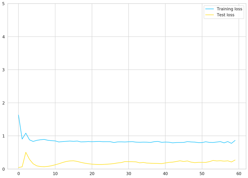

Our model’s performance doesn’t improve after 15 epochs or so. Recall that we have very little data. Maybe we shouldn’t trust our model that much?

Predicting daily cases

Our model can (due to the way we’ve trained it) predict only a single day in the future. We’ll employ a simple strategy to overcome this limitation. Use predicted values as input for predicting the next days:

1with torch.no_grad():
2  test_seq = X_test[:1]
3  preds = []
4  for _ in range(len(X_test)):
5    y_test_pred = model(test_seq)
6    pred = torch.flatten(y_test_pred).item()
7    preds.append(pred)
8    new_seq = test_seq.numpy().flatten()
9    new_seq = np.append(new_seq, [pred])
10    new_seq = new_seq[1:]
11    test_seq = torch.as_tensor(new_seq).view(1, seq_length, 1).float()

We have to reverse the scaling of the test data and the model predictions:

1true_cases = scaler.inverse_transform(
2    np.expand_dims(y_test.flatten().numpy(), axis=0)
3).flatten()
4
5predicted_cases = scaler.inverse_transform(
6  np.expand_dims(preds, axis=0)
7).flatten()

Let’s look at the results:

1plt.plot(
2  daily_cases.index[:len(train_data)],
3  scaler.inverse_transform(train_data).flatten(),
4  label='Historical Daily Cases'
5)
6
7plt.plot(
8  daily_cases.index[len(train_data):len(train_data) + len(true_cases)],
9  true_cases,
10  label='Real Daily Cases'
11)
12
13plt.plot(
14  daily_cases.index[len(train_data):len(train_data) + len(true_cases)],
15  predicted_cases,
16  label='Predicted Daily Cases'
17)
18
19plt.legend();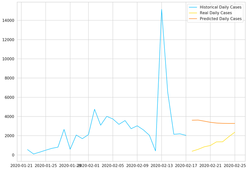

As expected, our model doesn’t perform very well. That said, the predictions seem to be in the right ballpark (probably due to using the last data point as a strong predictor for the next).

Use all data for training

Now, we’ll use all available data to train the same model:

1scaler = MinMaxScaler()
2
3scaler = scaler.fit(np.expand_dims(daily_cases, axis=1))
4
5all_data = scaler.transform(np.expand_dims(daily_cases, axis=1))
6
7all_data.shape

1(41, 1)

The preprocessing and training steps are the same:

1X_all, y_all = create_sequences(all_data, seq_length)
2
3X_all = torch.from_numpy(X_all).float()
4y_all = torch.from_numpy(y_all).float()
5
6model = CoronaVirusPredictor(
7  n_features=1,
8  n_hidden=512,
9  seq_len=seq_length,
10  n_layers=2
11)
12model, train_hist, _ = train_model(model, X_all, y_all)

1Epoch 0 train loss: 1.9441421031951904
2Epoch 10 train loss: 0.8385428786277771
3Epoch 20 train loss: 0.8256545066833496
4Epoch 30 train loss: 0.8023681640625
5Epoch 40 train loss: 0.8125611543655396
6Epoch 50 train loss: 0.8225002884864807

Predicting future cases

We’ll use our “fully trained” model to predict the confirmed cases for 12 days into the future:

1DAYS_TO_PREDICT = 12
2
3with torch.no_grad():
4  test_seq = X_all[:1]
5  preds = []
6  for _ in range(DAYS_TO_PREDICT):
7    y_test_pred = model(test_seq)
8    pred = torch.flatten(y_test_pred).item()
9    preds.append(pred)
10    new_seq = test_seq.numpy().flatten()
11    new_seq = np.append(new_seq, [pred])
12    new_seq = new_seq[1:]
13    test_seq = torch.as_tensor(new_seq).view(1, seq_length, 1).float()

As before, we’ll inverse the scaler transformation:

1predicted_cases = scaler.inverse_transform(
2  np.expand_dims(preds, axis=0)
3).flatten()

To create a cool chart with the historical and predicted cases, we need to extend the date index of our data frame:

1daily_cases.index[-1]

1Timestamp('2020-03-02 00:00:00')

1predicted_index = pd.date_range(
2  start=daily_cases.index[-1],
3  periods=DAYS_TO_PREDICT + 1,
4  closed='right'
5)
6
7predicted_cases = pd.Series(
8  data=predicted_cases,
9  index=predicted_index
10)
11
12plt.plot(predicted_cases, label='Predicted Daily Cases')
13plt.legend();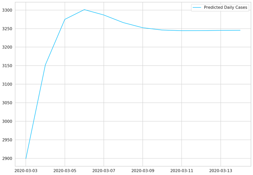

Now we can use all the data to plot the results:

1plt.plot(daily_cases, label='Historical Daily Cases')
2plt.plot(predicted_cases, label='Predicted Daily Cases')
3plt.legend();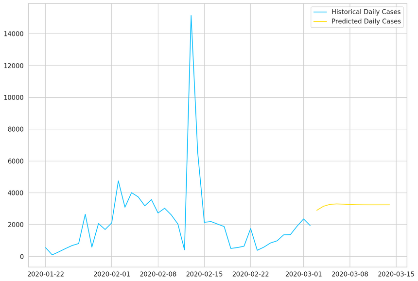

Our model thinks that things will level off. Note that the more you go into the future, the more you shouldn’t trust your model predictions.

Conclusion

Well done! You learned how to use PyTorch to create a Recurrent Neural Network that works with Time Series data. The model performance is not that great, but this is expected, given the small amounts of data.

The problem of predicting daily Covid-19 cases is a hard one. We’re amidst an outbreak, and there’s more to be done. Hopefully, everything will be back to normal after some time.

References

Want to be a Machine Learning expert?

Join the weekly newsletter on Data Science, Deep Learning and Machine Learning in your inbox, curated by me! Chosen by 10,000+ Machine Learning practitioners. (There might be some exclusive content, too!)

You'll never get spam from me

Hacker's Guide to Neural Networks in JavaScript

Build Machine Learning models (especially Deep Neural Networks) that you can easily integrate with existing or new web apps. Think of your ReactJs, Vue, or Angular app enhanced with the power of Machine Learning models.

Get SH*T Done with PyTorch

Learn how to solve real-world problems with Deep Learning models (NLP, Computer Vision, and Time Series). Go from prototyping to deployment with PyTorch and Python!

Hacker's Guide to Machine Learning with Python

This book brings the fundamentals of Machine Learning to you, using tools and techniques used to solve real-world problems in Computer Vision, Natural Language Processing, and Time Series analysis. The skills taught in this book will lay the foundation for you to advance your journey to Machine Learning Mastery!

Hands-On Machine Learning from Scratch

This book will guide you on your journey to deeper Machine Learning understanding by developing algorithms in Python from scratch! Learn why and when Machine learning is the right tool for the job and how to improve low performing models!