TL;DR Learn about Time Series and making predictions using Recurrent Neural Networks. Prepare sequence data and use LSTMs to make simple predictions.

Often you might have to deal with data that does have a time component. No matter how much you squint your eyes, it will be difficult to make your favorite data independence assumption. It seems like newer values in your data might depend on the historical values. How can you use that kind of data to build models?

This guide will help you better understand Time Series data and how to build models using Deep Learning (Recurrent Neural Networks). You’ll learn how to preprocess Time Series, build a simple LSTM model, train it, and use it to make predictions. Here are the steps:

• Time Series
• Recurrent Neural Networks
• Time Series Prediction with LSTMs

Run the complete notebook in your browser

The complete project on GitHub

Time Series

Time Series is a collection of data points indexed based on the time they were collected. Most often, the data is recorded at regular time intervals. What makes Time Series data special?

Forecasting future Time Series values is a quite common problem in practice. Predicting the weather for the next week, the price of Bitcoins tomorrow, the number of your sales during Chrismas and future heart failure are common examples.

Time Series data introduces a “hard dependency” on previous time steps, so the assumption that independence of observations doesn’t hold. What are some of the properties that a Time Series can have?

Stationarity, seasonality, and autocorrelation are some of the properties of the Time Series you might be interested in.

A Times Series is said to be stationary when the mean and variance remain constant over time. A Time Series has a trend if the mean is varying over time. Often you can eliminate it and make the series stationary by applying log transformation(s).

Seasonality refers to the phenomenon of variations at specific time-frames. eg people buying more Christmas trees during Christmas (who would’ve thought). A common approach to eliminating seasonality is to use differencing.

Autocorrelation refers to the correlation between the current value with a copy from a previous time (lag).

Why we would want to seasonality, trend and have a stationary Time Series? This is required data preprocessing step for Time Series forecasting with classical methods like ARIMA models. Luckily, we’ll do our modeling using Recurrent Neural Networks.

Recurrent Neural Networks

Recurrent neural networks (RNNs) can predict the next value(s) in a sequence or classify it. A sequence is stored as a matrix, where each row is a feature vector that describes it. Naturally, the order of the rows in the matrix is important.

RNNs are a really good fit for solving Natural Language Processing (NLP) tasks where the words in a text form sequences and their position matters. That said, cutting edge NLP uses the Transformer for most (if not all) tasks.

As you might’ve already guessed, Time Series is just one type of a sequence. We’ll have to cut the Time Series into smaller sequences, so our RNN models can use them for training. But how do we train RNNs?

First, let’s develop an intuitive understanding of what recurrent means. RNNs contain loops. Each unit has a state and receives two inputs - states from the previous layer and the stats from this layer from the previous time step.

The Backpropagation algorithm breaks down when applied to RNNs because of the recurrent connections. Unrolling the network, where copies of the neurons that have recurrent connections are created, can solve this problem. This converts the RNN into a regular Feedforward Neural Net, and classic Backpropagation can be applied. The modification is known as Backpropagation through time.

Problems with Classical RNNs

Unrolled Neural Networks can get very deep (that’s what he said), which creates problems for the gradient calculations. The weights can become very small (Vanishing gradient problem) or very large (Exploding gradient problem).

Classic RNNs also have a problem with their memory (long-term dependencies), too. The begging of the sequences we use for training tends to be “forgotten” because of the overwhelming effect of more recent states.

In practice, those problems are solved by using gated RNNs. They can store information for later use, much like having a memory. Reading, writing, and deleting from the memory are learned from the data. The two most commonly used gated RNNs are Long Short-Term Memory Networks and Gated Recurrent Unit Neural Networks.

Time Series Prediction with LSTMs

We’ll start with a simple example of forecasting the values of the Sine function using a simple LSTM network.

Setup

Let’s start with the library imports and setting seeds:

1import numpy as np
2import tensorflow as tf
3from tensorflow import keras
4import pandas as pd
5import seaborn as sns
6from pylab import rcParams
7import matplotlib.pyplot as plt
8from matplotlib import rc
9
10%matplotlib inline
11%config InlineBackend.figure_format='retina'
12
13sns.set(style='whitegrid', palette='muted', font_scale=1.5)
14
15rcParams['figure.figsize'] = 16, 10
16
17RANDOM_SEED = 42
18
19np.random.seed(RANDOM_SEED)
20tf.random.set_seed(RANDOM_SEED)

Data

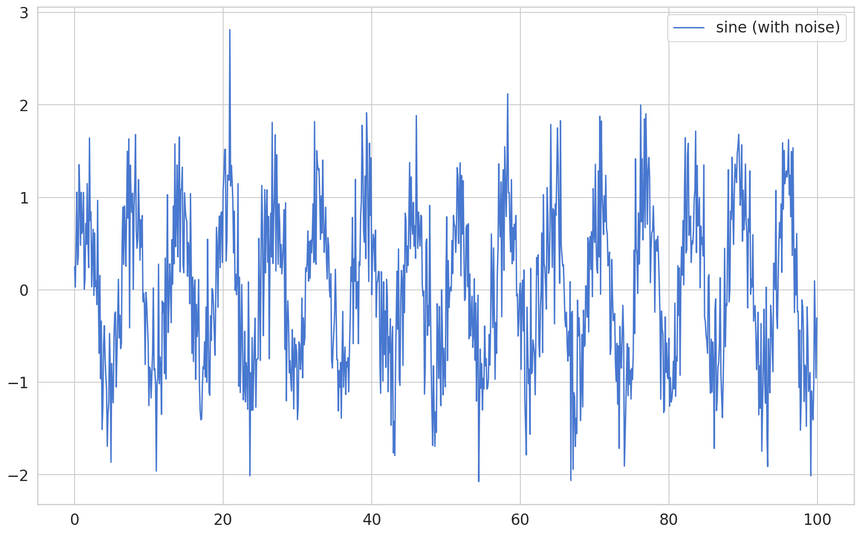
We’ll generate 1,000 values from the sine function and use that as training data. But, we’ll add a little bit of zing to it:

1time = np.arange(0, 100, 0.1)
2sin = np.sin(time) + np.random.normal(scale=0.5, size=len(time))

A random value, drawn from a normal distribution, is added to each data point. That’ll make the job of our model a bit harder.

Data Preprocessing

We need to “chop the data” into smaller sequences for our model. But first, we’ll split it into training and test data:

1df = pd.DataFrame(dict(sine=sin), index=time, columns=['sine'])
2
3train_size = int(len(df) * 0.8)
4test_size = len(df) - train_size
5train, test = df.iloc[0:train_size], df.iloc[train_size:len(df)]
6print(len(train), len(test))

1800 200

Preparing the data for Time Series forecasting (LSTMs in particular) can be tricky. Intuitively, we need to predict the value at the current time step by using the history (n time steps from it). Here’s a generic function that does the job:

1def create_dataset(X, y, time_steps=1):
2    Xs, ys = [], []
3    for i in range(len(X) - time_steps):
4        v = X.iloc[i:(i + time_steps)].values
5        Xs.append(v)
6        ys.append(y.iloc[i + time_steps])
7    return np.array(Xs), np.array(ys)

The beauty of this function is that it works with univariate (single feature) and multivariate (multiple features) Time Series data. Let’s use a history of 10 time steps to make our sequences:

1time_steps = 10
2
3# reshape to [samples, time_steps, n_features]
4
5X_train, y_train = create_dataset(train, train.sine, time_steps)
6X_test, y_test = create_dataset(test, test.sine, time_steps)
7
8print(X_train.shape, y_train.shape)

1(790, 10, 1) (790,)

We have our sequences in the shape (samples, time_steps, features). How can we use them to make predictions?

Modeling

Training an LSTM model in Keras is easy. We’ll use the LSTM layer in a sequential model to make our predictions:

1model = keras.Sequential()
2model.add(keras.layers.LSTM(
3  units=128,
4  input_shape=(X_train.shape[1], X_train.shape[2])
5))
6model.add(keras.layers.Dense(units=1))
7model.compile(
8  loss='mean_squared_error',
9  optimizer=keras.optimizers.Adam(0.001)
10)

The LSTM layer expects the number of time steps and the number of features to work properly. The rest of the model looks like a regular regression model. How do we train a LSTM model?

Training

The most important thing to remember when training Time Series models is to not shuffle the data (the order of the data matters). The rest is pretty standard:

1history = model.fit(
2    X_train, y_train,
3    epochs=30,
4    batch_size=16,
5    validation_split=0.1,
6    verbose=1,
7    shuffle=False
8)

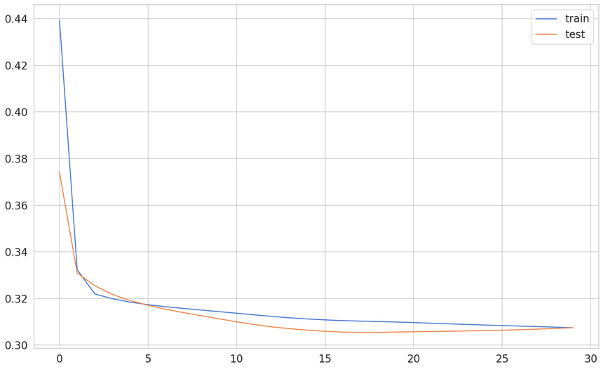
Our dataset is pretty simple and contains the randomness from our sampling. After about 15 epochs, the model is pretty much-done learning.

Evaluation

Let’s take some predictions from our model:

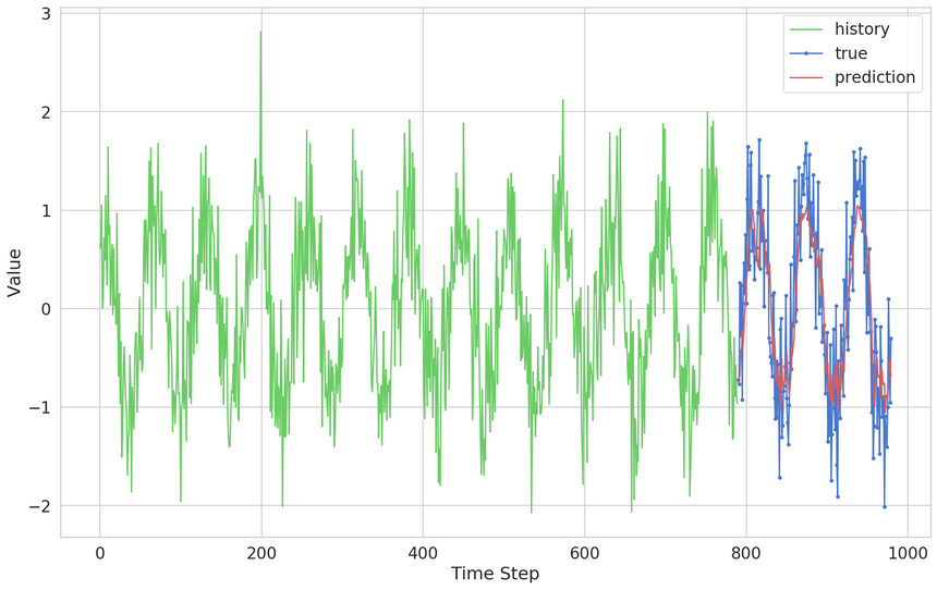
1y_pred = model.predict(X_test)

We can plot the predictions over the true values from the Time Series:

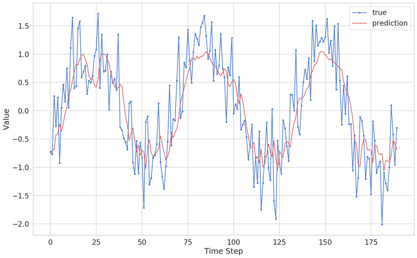
Our predictions look really good on this scale. Let’s zoom in:

The model seems to be doing a great job of capturing the general pattern of the data. It fails to capture random fluctuations, which is a good thing (it generalizes well).

Conclusion

Congratulations! You made your first Recurrent Neural Network model! You also learned how to preprocess Time Series data, something that trips a lot of people.

• Time Series
• Recurrent Neural Networks
• Time Series Prediction with LSTMs

We’ve just scratched the surface of Time Series data and how to use Recurrent Neural Networks. Some interesting applications are Time Series forecasting, (sequence) classification and anomaly detection. The fun part is just getting started!

Run the complete notebook in your browser

The complete project on GitHub

References

• TensorFlow - Time series forecasting
• Understanding LSTM Networks