Curiousily

TL;DR Learn how to implement Gradient Descent for cases with multiple features in your dataset. Understand how Backpropagation work and use it together with Gradient Descent to train a Deep Neural Network.

You’re still trying to build a model that predicts the number of infected patients (with a novel respiratory virus) for tomorrow based on historical data. But now, you have more data. You’re ready to use a more powerful model - Deep Neural Network.

• Run the complete source code on CodeSandbox

In this part, you’ll learn how to:

• Implement Generalized Gradient Descent and train a small Neural Network with it
• Learn how Backpropagation works and implement it from scratch using TensorFlow.js
• Train a Deep Neural Network using Backpropagation to predict the number of infected patients

If you’re thinking about skipping this part - DON’T! You should really understand how Backpropagation works!

In the previous part, you’ve implemented gradient descent for a single input. Can we do the same with multiple features?

A feature is a characteristic of each example in your dataset. For example - if you want to predict somebody`s age you might have features like height, weight and gender.

Generalized Gradient Descent

Let’s start with a review of the data that you’ll use to train our Neural Network:

1const DATA = [
2  // infections, infected countries
3  [2.0, 1.0],
4  [5.0, 1.0],
5  [7.0, 4.0],
6  [12.0, 5.0],
7]
8
9const nextDayInfections = [5.0, 7.0, 12.0, 19.0]

We have two features this time around - the number of daily infections and the number of countries with infected patients.

Let’s create the initial weight values. We’ll use 2 - one for each feature:

1var weights = [1.0, 0.5]

How I come up with the values? I just spit out some numbers. Is this the best you can do? No! In fact, choosing good initial weight values is really important. We’ll look at a simple and good strategy to do it in the next section.

Your simple Neural Network looks like this:

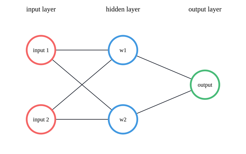
You already know how to make predictions when you have multiple inputs - take the weighted sum of a data point and the weights:

1const weightedSum = (data, weights) => {
2  var prediction = 0
3  for (const [i, weight] of weights.entries()) {
4    prediction += data[i] * weight
5  }
6  return prediction
7}
8
9const neuralNet = (data, weights) => weightedSum(data, weights)

We also need to adjust our method for updating the weights (since we have more than one). You need to apply the update rule for each feature and its associated weight:

1const updateWeights = (dataPoint, prediction, trueInfectedCount) => {
2  for (const [i, d] of dataPoint.entries()) {
3    const update = (prediction - trueInfectedCount) * d
4    weights[i] -= ALPHA * update
5  }
6}

Alright, you now have all the components to implement the generalized version of Gradient Descent:

1const ALPHA = 0.0002
2
3const DATA = [
4  // infections, infected countries
5  [2.0, 1.0],
6  [5.0, 1.0],
7  [7.0, 4.0],
8  [12.0, 5.0],
9]
10
11const nextDayInfections = [5.0, 7.0, 12.0, 19.0]
12
13var weights = [1.0, 0.5]
14
15const weightedSum = (data, weights) => {
16  var prediction = 0
17
18  for (const [i, weight] of weights.entries()) {
19    prediction += data[i] * weight
20  }
21
22  return prediction
23}
24
25const updateWeights = (dataPoint, prediction, trueInfectedCount) => {
26  for (const [i, d] of dataPoint.entries()) {
27    const update = (prediction - trueInfectedCount) * d
28    weights[i] -= ALPHA * update
29  }
30}
31
32const neuralNet = (data, weights) => weightedSum(data, weights)
33const error = (prediction, trueValue) => (prediction - trueValue) ** 2
34
35for (const i of Array(100).keys()) {
36  var errors = 0
37
38  console.log(`epoch ${i + 1}`)
39
40  for (const [j, dataPoint] of DATA.entries()) {
41    const prediction = neuralNet(dataPoint, weights)
42    const trueInfectedCount = nextDayInfections[j]
43
44    errors += error(prediction, trueInfectedCount)
45
46    updateWeights(dataPoint, prediction, trueInfectedCount)
47
48    console.log(`prediction: ${prediction}`)
49  }
50
51  const epochError = errors / DATA.length
52  console.log(`error: ${epochError}\n`)
53}

1epoch 1
2prediction: 2.5
3prediction: 5.505499999999999
4prediction: 9.020657099999998
5prediction: 14.59589883232
6error: 9.189030365235194
7
8epoch 2
9prediction: 2.5420573212125435
10prediction: 5.599171063693172
11prediction: 9.17076892133457
12prediction: 14.836072301932777
13error: 8.336661573054283
14
15epoch 3
16prediction: 2.5819331000831913
17prediction: 5.687974183830248
18prediction: 9.313097463682844
19prediction: 15.063781754512572
20error: 7.570429647636219
21
22...
23
24epoch 98
25prediction: 3.307142155409998
26prediction: 7.289664016823003
27prediction: 11.906137672497662
28prediction: 19.196247772845233
29error: 0.7492490623757035
30
31epoch 99
32prediction: 3.307397419714084
33prediction: 7.2900623947196825
34prediction: 11.907106811690227
35prediction: 19.19759306027421
36error: 0.7491779623809854
37
38epoch 100
39prediction: 3.3076402607543107
40prediction: 7.29043311877873
41prediction: 11.90803160421936
42prediction: 19.198867413412678
43error: 0.7491098293607978

The error is gradually (pun intended) reducing - great! We iterate over each data point, make a prediction, calculate the error and adjust the weights.

We did get the job done but that code took an awful lot lines to write. Let’s look at the same implementation using TensorFlow.js:

1import * as tf from "@tensorflow/tfjs"
2
3const ALPHA = 0.0002
4
5const DATA = tf.tensor([
6  // infections, infected countries
7  [2.0, 1.0],
8  [5.0, 1.0],
9  [7.0, 4.0],
10  [12.0, 5.0],
11])
12
13const nextDayInfections = tf.tensor([5.0, 7.0, 12.0, 19.0])
14
15var weights = tf.tensor([1.0, 0.5])
16
17const neuralNet = (data, weights) => data.dot(weights)
18const error = (prediction, trueValue) => tf.square(prediction.sub(trueValue))
19
20for (const i of Array(100).keys()) {
21  const prediction = neuralNet(DATA, weights)
22
23  const epochError = tf.mean(error(prediction, nextDayInfections))
24
25  const loss = prediction.sub(nextDayInfections)
26
27  const change = loss.dot(DATA).mul(ALPHA)
28
29  weights = weights.sub(change)
30
31  console.log(`epoch ${i + 1}`)
32
33  for (const n of prediction.dataSync()) {
34    console.log(`prediction: ${n.toFixed(2)}`)
35  }
36
37  console.log(`error: ${epochError.dataSync()}\n`)
38}

1epoch 1
2prediction: 2.50
3prediction: 5.50
4prediction: 9.00
5prediction: 14.50
6error: 9.4375
7
8epoch 2
9prediction: 2.54
10prediction: 5.60
11prediction: 9.15
12prediction: 14.75
13error: 8.547682762145996
14
15epoch 3
16prediction: 2.58
17prediction: 5.69
18prediction: 9.30
19prediction: 14.98
20error: 7.74901819229126
21
22...
23
24epoch 98
25prediction: 3.31
26prediction: 7.29
27prediction: 11.91
28prediction: 19.20
29error: 0.7479317784309387
30
31epoch 99
32prediction: 3.31
33prediction: 7.29
34prediction: 11.91
35prediction: 19.20
36error: 0.7478666305541992
37
38epoch 100
39prediction: 3.31
40prediction: 7.29
41prediction: 11.91
42prediction: 19.20
43error: 0.7478042244911194

Much more succint! Calculating the weighted sum and updating the weights is done by using a couple of Tensor methods. The results are pretty much the same.

You migh’ve noticed something else here. Why don’t we iterate over the examples of our dataset? TensorFlow.js is utilizing a technique called vectorization:

“Vectorization” (simplified) is the process of rewriting a loop so that instead of processing a single element of an array N times, it processes (say) 4 elements of the array simultaneously N/4 times. Stephen Canon

So, TensorFlow.js makes things faster and easier to read! There are a lot of frameworks that can do that for you, but in JavaScript land TensorFlow.js is king! So, TensorFlow.js makes things faster and easier to read!

Backpropagation

Backpropagation is an algorithm for training Neural Networks. Given the current error, Backpropagation figures out how much each weight contributes to this error and the amount that needs to be changed (using gradients). It works with arbitrarily complex Neural Nets!

Backpropagation doesn’t update (optimize) the weights! For that, you need optimization algorithms such as Gradient Descent.

Alright, but we did pretty well without Backpropagation so far? Why use it? Well, you’ve been using Backpropagation all along. Your Neural Network was just… tiny!

Training a Deep Neural Network with Backpropagation

In recent years, Deep Neural Networks beat pretty much every other model on various Machine Learning tasks. They are like the crazy hottie you’re so much attracted to - can give you immense pleasure but can also make your life miserable if left unchecked.

They are extremely flexible models, but so much choice comes with a price. Sometimes, you don’t know which option is best. A variety of tools, libraries, architectures, optimizers, bizarre ideas has exploded recently. How can you choose?

I’ll use the Lindy effect and show you concepts that stood the test of time. Later on, you’ll build a complete Deep Neural Network and train it with Backpropagation!

The Lindy effect is a theory that the future life expectancy of some non-perishable things like a technology or an idea is proportional to their current age, so that every additional period of survival implies a longer remaining life expectancy. Lindy effect - Wikipedia

Deep Neural Networks

The intuition behind Artificial Neural Network (ANNs) models can be explained by squinting your eyes and looking at how our brains work and their structure. Our brains contain neurons (weights) and connections (synapses).

In ANNs, weights are arranged in horizontal structures known as layers. Layers are stacked over each other. But why?

Neural Networks contain input layers (where the data gets fed), hidden layer(s) (parameters (weights) that are learned during training), and an output layer (the predicted value(s)). Neural Networks with 2 or more (hidden) layers are called Deep Neural Networks

Neural Networks are very good nonlinear learners - they can approximate functions that are not representable with a line. This is possible by stacking layers. In the real world - not very many problems can be solved by drawing a line (e.g. predicting car prices by a linear relationship will not give you a good result - some cars are much more expensive than your linear model expects). How can they do that?

Activation functions

Introducing nonlinearity in your Neural Network is achieved by adding activation functions to each layer’s output.

Building a Neural Network with multiple layers without adding activation functions between them is equivalent to building a Neural Network with a single layer.

Let’s try to stack (call one with the result from another) two linear functions:

and

Combining those two gives you a new function:

The result is still a linear function. Have a look:

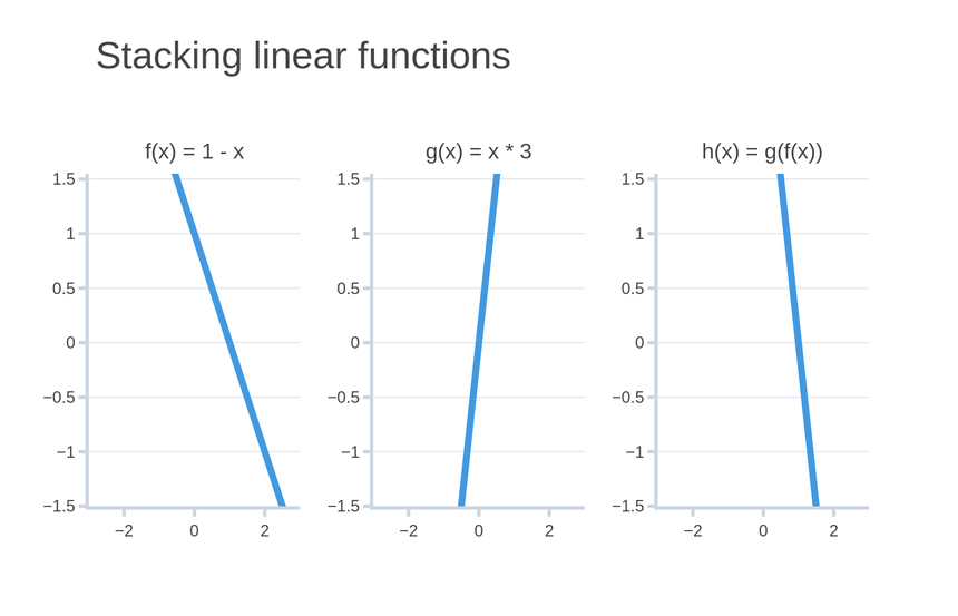
And here’s a preview of what stacking nonlinear functions looks like:

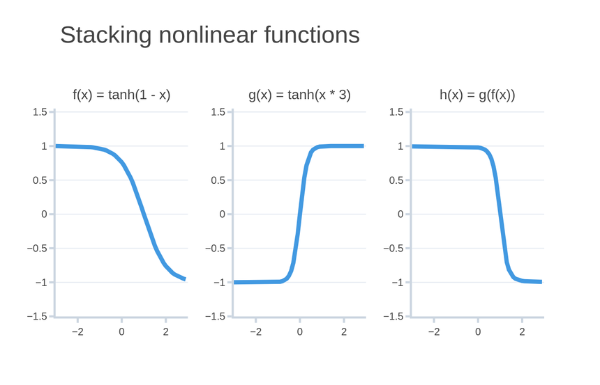
Alright, those activation functions sound really magical. They must be hard to understand and implement, right? Not at all!

Let’s look at one that you might already be familiar with - the hyperbolic tangent:

And here is the TensorFlow.js version:

1const tanh = x => tf.sinh(x).div(tf.cosh(x))

We’re also going to use the first derivative of $\tanh$. Here is the definition (taken from a table of derivates):

The implementation creates a tensor of ones (with the correct shape) and substracts the squared $\tanh$ from it:

1const tanhPrime = x => tf.ones(x.shape).sub(tf.square(tanh(x)))

If you are anything like me, this will not give you a clear picture of what is happening. So here is one that should do it:

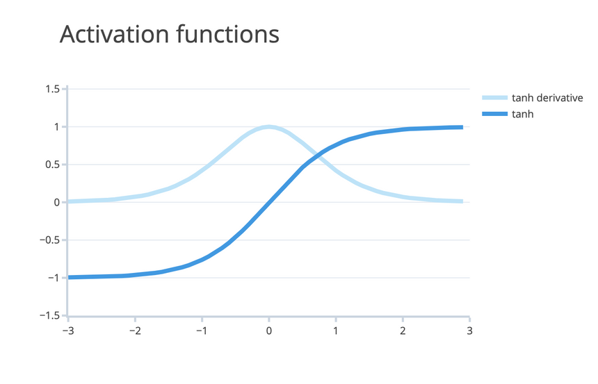
Weight initialization

Thus far, the weights we’ve been using have been somewhat of magic numbers. What initial values are good for our weights?

For quite a while, Neural Networks and other models “weren’t working” during the 80s and 90s. Almost all hopes were lost. Those periods are known as AI Winters. What were the reasons?

For one, the hardware wasn’t quite there - you simply couldn’t process and store large amounts of high-quality images and texts. Also, the algorithms weren’t quite effective! Weight initialization was also a problem - what values should we use?

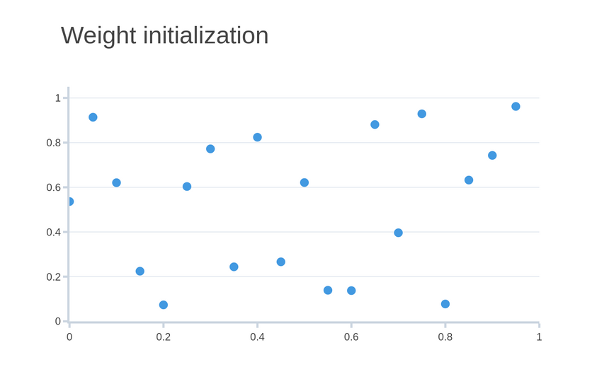
Turns out (found with mostly empirical testing) weights must be initialized with small random numbers. This is mostly due to the quirks of using Gradient Descent - starting from random locations in high dimensional spaces lets you explore more possibilities for good weights (low errors) as the algorithm does its magic.

In practice, we can use values from a uniform distribution in TensorFlow.js like so:

1const weights = tf.randomUniform([100], 0, 1)

This generates 100 values in the range between 0 and 1. Here is how they might look:

Architecture

We’ll train a Deep Neural Network with 2 layers. Let’s start by converting the data to Tensors:

1const DATA = tf.tensor([
2  // infections, infected countries
3  [2.0, 1.0],
4  [5.0, 1.0],
5  [7.0, 4.0],
6  [12.0, 5.0],
7])
8
9const nextDayInfections = tf.expandDims(tf.tensor([5.0, 7.0, 12.0, 19.0]), 1)

Note that we convert the next day infections to 2D tensor (using expandDims()). This will make the code much more readable.

We need two sets of weights (for each hidden layer):

1const HIDDEN_SIZE = 4
2
3var weights1 = tf.randomUniform([2, HIDDEN_SIZE], 0, 1)
4var weights2 = tf.randomUniform([HIDDEN_SIZE, 1], 0, 1)

Here’s how your Deep Neural Net looks like:

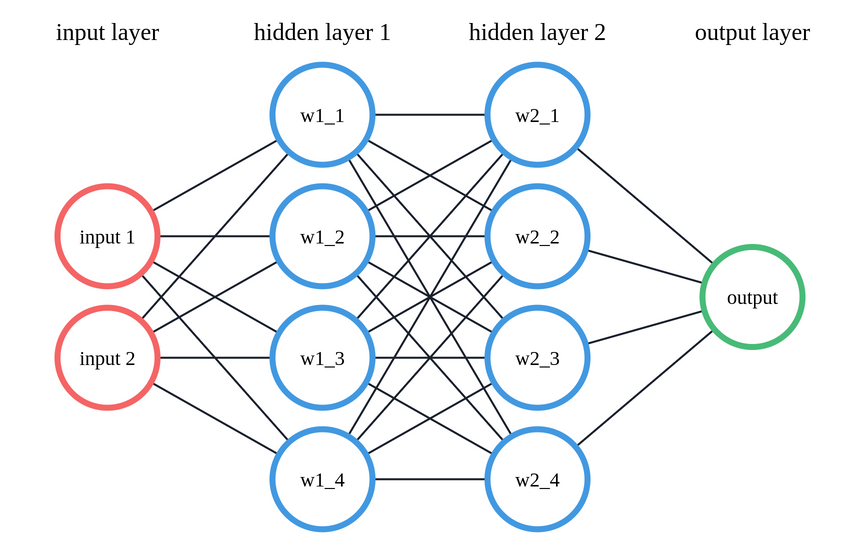
Our input layer has a size of 2 - infections and infected countries. This gets connected to the first hidden layer with 4 neurons. The second hidden layer also contains 4 neurons. It gets connected to the output layer with a size of 1 (the number of predicted infections for tomorrow).

Finally, we can run the Backpropagation algorithm:

1const layer1 = tanh(DATA.dot(weights1))
2const layer2 = layer1.dot(weights2)
3
4const layer2Delta = layer2.sub(nextDayInfections)
5const layer1Delta = layer2Delta.dot(weights2.transpose()).mul(tanhPrime(layer1))
6
7weights2 = weights2.sub(layer1.transpose().dot(layer2Delta).mul(ALPHA))
8weights1 = weights1.sub(DATA.transpose().dot(layer1Delta).mul(ALPHA))

We start by taking the weighted sum of the data and the weights of the first hidden layer. The result gets passed to our activation function tanh(). This is the prediction of the first hidden layer.

The prediction of the next hidden layer is simply the dot product (weighted sum) of the previous layer with the weights for the second hidden layer.

Next, we need to calculate how much each weight should be changed. We can do that by identifying how much each weight contributed to the error.

For the second hidden layer, we’re using the difference between the prediction and real values. That’s it!

The change of the first hidden layer is computed by taking the previous delta and multiplying it with the weights of the layer. Finally, we do element-wise multiplication with the first derivative of $\tanh$ to apply the rate of change given by the activation function.

The weight update rules are pretty much identical, except that we apply transpose() to convert the tensors into correct shapes so that operations can be applied correctly.

The weights of the second hidden layer get updates based on the weighted sum of the change (delta) and the prediction from the first hidden layer. The first hidden layer gets updated by using the original dataset.

Here is the complete example, running for 20 epochs:

1import * as tf from "@tensorflow/tfjs"
2
3const ALPHA = 0.01
4
5const HIDDEN_SIZE = 4
6
7const DATA = tf.tensor([
8  // infections, infected countries
9  [2.0, 1.0],
10  [5.0, 1.0],
11  [7.0, 4.0],
12  [12.0, 5.0],
13])
14
15const nextDayInfections = tf.expandDims(tf.tensor([5.0, 7.0, 12.0, 19.0]), 1)
16
17var weights1 = tf.randomUniform([2, HIDDEN_SIZE], 0, 1)
18var weights2 = tf.randomUniform([HIDDEN_SIZE, 1], 0, 1)
19
20const tanh = x => tf.sinh(x).div(tf.cosh(x))
21
22const tanhPrime = x => tf.ones(x.shape).sub(tf.square(tanh(x)))
23
24for (const i of Array(20).keys()) {
25  const layer1 = tanh(DATA.dot(weights1))
26  const layer2 = layer1.dot(weights2)
27
28  const layer2Delta = layer2.sub(nextDayInfections)
29  const layer1Delta = layer2Delta
30    .dot(weights2.transpose())
31    .mul(tanhPrime(layer1))
32
33  weights2 = weights2.sub(layer1.transpose().dot(layer2Delta).mul(ALPHA))
34
35  weights1 = weights1.sub(DATA.transpose().dot(layer1Delta).mul(ALPHA))
36
37  const currentError = tf.mean(tf.square(layer2.sub(nextDayInfections)))
38  console.log(`epoch ${i + 1} error: ${currentError.dataSync()}`)
39}

1epoch 1 error: 125.68846130371094
2epoch 2 error: 97.80104064941406
3epoch 3 error: 77.51105499267578
4epoch 4 error: 63.27639389038086
5...
6epoch 17 error: 29.5538330078125
7epoch 18 error: 29.44598388671875
8epoch 19 error: 29.36988639831543
9epoch 20 error: 29.316192626953125

Interestingly, that error is surely reducing but not hitting quite as low as before. Can you find out why?

Summary

Well, you surely learned a lot about how to train Neural Networks. The Backpropagation algorithm has been around for a long time and seems to be working quite well in practice. This part helps you understand how exactly is doing its thing.

• Run the complete source code on CodeSandbox

In this part, you learned how to:

• Implement Generalized Gradient Descent and train a small Neural Network with it
• Learn how Backpropagation works and implement it from scratch using TensorFlow.js
• Train a Deep Neural Network using Backpropagation to predict the number of infected patients

So, now you’re ready to create infinitely complex Deep Neural Nets that solve any problem, right? Of course not!

If you’re anything like me, you want to try out different alphas, activation functions, and architectures. And you might cringe when you think that you need to deal with derivatives of funky functions. Fortunately, TensorFlow.js gots you covered - it makes things really simple and hides most of the complexities associated with Deep Learning.

How easy could it be? I’ll show you next!

References

• A Neural Network in 11 lines of Python - Andrew Trask
• Why Initialize a Neural Network with Random Weights? - Jason Brownlee
• How the backpropagation algorithm works - Michael Nielsen