Curiousily

Transfer Learning for Image Classification using Torchvision, Pytorch and Python

24.05.2020 — Deep Learning, Computer Vision, Machine Learning, Neural Network, Transfer Learning, Python — 4 min read

TL;DR Learn how to use Transfer Learning to classify traffic sign images. You’ll build a dataset of images in a format suitable for working with Torchvision. Get predictions on images from the wild (downloaded from the Internet).

In this tutorial, you’ll learn how to fine-tune a pre-trained model for classifying raw pixels of traffic signs.

Here’s what we’ll go over:

Overview of the traffic sign image dataset
Build a dataset
Use a pre-trained model from Torchvision
Add a new unknown class and re-train the model

Will this model be ready for the real world?

1import torch, torchvision
2
3from pathlib import Path
4import numpy as np
5import cv2
6import pandas as pd
7from tqdm import tqdm
8import PIL.Image as Image
9import seaborn as sns
10from pylab import rcParams
11import matplotlib.pyplot as plt
12from matplotlib import rc
13from matplotlib.ticker import MaxNLocator
14from torch.optim import lr_scheduler
15from sklearn.model_selection import train_test_split
16from sklearn.metrics import confusion_matrix, classification_report
17from glob import glob
18import shutil
19from collections import defaultdict
20
21from torch import nn, optim
22
23import torch.nn.functional as F
24import torchvision.transforms as T
25from torchvision.datasets import ImageFolder
26from torch.utils.data import DataLoader
27from torchvision import models
28
29%matplotlib inline
30%config InlineBackend.figure_format='retina'
31
32sns.set(style='whitegrid', palette='muted', font_scale=1.2)
33
34HAPPY_COLORS_PALETTE = ["#01BEFE", "#FFDD00", "#FF7D00", "#FF006D", "#ADFF02", "#8F00FF"]
35
36sns.set_palette(sns.color_palette(HAPPY_COLORS_PALETTE))
37
38rcParams['figure.figsize'] = 12, 8
39
40RANDOM_SEED = 42
41np.random.seed(RANDOM_SEED)
42torch.manual_seed(RANDOM_SEED)
43
44device = torch.device("cuda" if torch.cuda.is_available() else "cpu")

Recognizing traffic signs

German Traffic Sign Recognition Benchmark (GTSRB) contains more than 50,000 annotated images of 40+ traffic signs. Given an image, you’ll have to recognize the traffic sign on it.

1!wget https://sid.erda.dk/public/archives/daaeac0d7ce1152aea9b61d9f1e19370/GTSRB_Final_Training_Images.zip
2!unzip -qq GTSRB_Final_Training_Images.zip

Exploration

Let’s start by getting a feel of the data. The images for each traffic sign are stored in a separate directory. How many do we have?

1train_folders = sorted(glob('GTSRB/Final_Training/Images/*'))
2len(train_folders)

We’ll create 3 helper functions that use OpenCV and Torchvision to load and show images:

1def load_image(img_path, resize=True):
2  img = cv2.cvtColor(cv2.imread(img_path), cv2.COLOR_BGR2RGB)
3
4  if resize:
5    img = cv2.resize(img, (64, 64), interpolation = cv2.INTER_AREA)
6
7  return img
8
9def show_image(img_path):
10  img = load_image(img_path)
11  plt.imshow(img)
12  plt.axis('off')
13
14def show_sign_grid(image_paths):
15  images = [load_image(img) for img in image_paths]
16  images = torch.as_tensor(images)
17  images = images.permute(0, 3, 1, 2)
18  grid_img = torchvision.utils.make_grid(images, nrow=11)
19  plt.figure(figsize=(24, 12))
20  plt.imshow(grid_img.permute(1, 2, 0))
21  plt.axis('off');

Let’s have a look at some examples for each traffic sign:

1sample_images = [np.random.choice(glob(f'{tf}/*ppm')) for tf in train_folders]
2show_sign_grid(sample_images)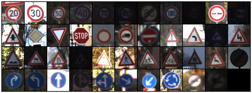

And here is a single sign:

1img_path = glob(f'{train_folders[16]}/*ppm')[1]
2
3show_image(img_path)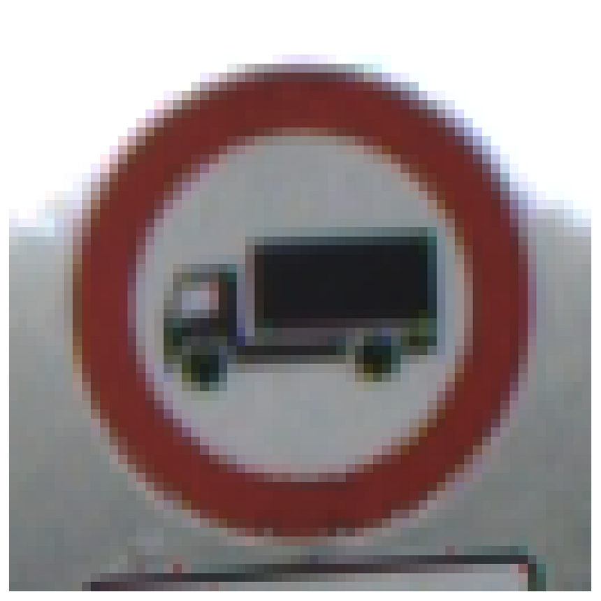

Building a dataset

To keep things simple, we’ll focus on classifying some of the most used traffic signs:

1class_names = ['priority_road', 'give_way', 'stop', 'no_entry']
2
3class_indices = [12, 13, 14, 17]

We’ll copy the images files to a new directory, so it’s easier to use the Torchvision’s dataset helpers. Let’s start with the directories for each class:

1!rm -rf data
2
3DATA_DIR = Path('data')
4
5DATASETS = ['train', 'val', 'test']
6
7for ds in DATASETS:
8  for cls in class_names:
9    (DATA_DIR / ds / cls).mkdir(parents=True, exist_ok=True)

We’ll reserve 80% of the images for training, 10% for validation, and 10% test for each class. We’ll copy each image to the correct dataset directory:

1for i, cls_index in enumerate(class_indices):
2  image_paths = np.array(glob(f'{train_folders[cls_index]}/*.ppm'))
3  class_name = class_names[i]
4  print(f'{class_name}: {len(image_paths)}')
5  np.random.shuffle(image_paths)
6
7  ds_split = np.split(
8    image_paths,
9    indices_or_sections=[int(.8*len(image_paths)), int(.9*len(image_paths))]
10  )
11
12  dataset_data = zip(DATASETS, ds_split)
13
14  for ds, images in dataset_data:
15    for img_path in images:
16      shutil.copy(img_path, f'{DATA_DIR}/{ds}/{class_name}/')

1priority_road: 2100
2    give_way: 2160
3    stop: 780
4    no_entry: 1110

We have some class imbalance, but it is not that bad. We’ll ignore it.

We’ll apply some image augmentation techniques to artificially increase the size of our training dataset:

1mean_nums = [0.485, 0.456, 0.406]
2std_nums = [0.229, 0.224, 0.225]
3
4transforms = {'train': T.Compose([
5  T.RandomResizedCrop(size=256),
6  T.RandomRotation(degrees=15),
7  T.RandomHorizontalFlip(),
8  T.ToTensor(),
9  T.Normalize(mean_nums, std_nums)
10]), 'val': T.Compose([
11  T.Resize(size=256),
12  T.CenterCrop(size=224),
13  T.ToTensor(),
14  T.Normalize(mean_nums, std_nums)
15]), 'test': T.Compose([
16  T.Resize(size=256),
17  T.CenterCrop(size=224),
18  T.ToTensor(),
19  T.Normalize(mean_nums, std_nums)
20]),
21}

We apply some random resizing, rotation, and horizontal flips. Finally, we normalize the tensors using preset values for each channel. This is a requirement of the pre-trained models in Torchvision.

We’ll create a PyTorch dataset for each image dataset folder and data loaders for easier training:

1image_datasets = {
2  d: ImageFolder(f'{DATA_DIR}/{d}', transforms[d]) for d in DATASETS
3}
4
5data_loaders = {
6  d: DataLoader(image_datasets[d], batch_size=4, shuffle=True, num_workers=4)
7  for d in DATASETS
8}

We’ll also store the number of examples in each dataset and class names for later:

1dataset_sizes = {d: len(image_datasets[d]) for d in DATASETS}
2class_names = image_datasets['train'].classes
3
4dataset_sizes

1{'test': 615, 'train': 4920, 'val': 615}

Let’s have a look at some example images with applied transformations. We also need to reverse the normalization and reorder the color channels to get correct image data:

1def imshow(inp, title=None):
2  inp = inp.numpy().transpose((1, 2, 0))
3  mean = np.array([mean_nums])
4  std = np.array([std_nums])
5  inp = std * inp + mean
6  inp = np.clip(inp, 0, 1)
7  plt.imshow(inp)
8  if title is not None:
9    plt.title(title)
10  plt.axis('off')
11
12inputs, classes = next(iter(data_loaders['train']))
13out = torchvision.utils.make_grid(inputs)
14
15imshow(out, title=[class_names[x] for x in classes])

Using a pre-trained model:

Our model will receive raw image pixels and try to classify them into one of four traffic signs. How hard can it be? Try to build a model from scratch.

Here, we’ll use Transfer Learning to copy the architecture of the very popular ResNet model. On top of that, we’ll use the learned weights of the model from training on the ImageNet dataset . All of this is made easy to use by Torchvision:

1def create_model(n_classes):
2  model = models.resnet34(pretrained=True)
3
4  n_features = model.fc.in_features
5  model.fc = nn.Linear(n_features, n_classes)
6
7  return model.to(device)

We reuse almost everything except the change of the output layer. This is needed because the number of classes in our dataset is different than ImageNet.

Let’s create an instance of our model:

1base_model = create_model(len(class_names))

Training

We’ll write 3 helper functions to encapsulate the training and evaluation logic. Let’s start with train_epoch:

1def train_epoch(
2  model,
3  data_loader,
4  loss_fn,
5  optimizer,
6  device,
7  scheduler,
8  n_examples
9):
10  model = model.train()
11
12  losses = []
13  correct_predictions = 0
14
15  for inputs, labels in data_loader:
16    inputs = inputs.to(device)
17    labels = labels.to(device)
18
19    outputs = model(inputs)
20
21    _, preds = torch.max(outputs, dim=1)
22    loss = loss_fn(outputs, labels)
23
24    correct_predictions += torch.sum(preds == labels)
25    losses.append(loss.item())
26
27    loss.backward()
28    optimizer.step()
29    optimizer.zero_grad()
30
31  scheduler.step()
32
33  return correct_predictions.double() / n_examples, np.mean(losses)

We start by turning our model into train mode and go over the data. After getting the predictions, we get the class with maximum probability along with the loss, so we can calculate the epoch loss and accuracy.

Note that we’re also using a learning rate scheduler (more on that later).

1def eval_model(model, data_loader, loss_fn, device, n_examples):
2  model = model.eval()
3
4  losses = []
5  correct_predictions = 0
6
7  with torch.no_grad():
8    for inputs, labels in data_loader:
9      inputs = inputs.to(device)
10      labels = labels.to(device)
11
12      outputs = model(inputs)
13
14      _, preds = torch.max(outputs, dim=1)
15
16      loss = loss_fn(outputs, labels)
17
18      correct_predictions += torch.sum(preds == labels)
19      losses.append(loss.item())
20
21  return correct_predictions.double() / n_examples, np.mean(losses)

The evaluation of the model is pretty similar, except that we don’t do any gradient calculations.

Let’s put everything together:

1def train_model(model, data_loaders, dataset_sizes, device, n_epochs=3):
2  optimizer = optim.SGD(model.parameters(), lr=0.001, momentum=0.9)
3  scheduler = lr_scheduler.StepLR(optimizer, step_size=7, gamma=0.1)
4  loss_fn = nn.CrossEntropyLoss().to(device)
5
6  history = defaultdict(list)
7  best_accuracy = 0
8
9  for epoch in range(n_epochs):
10
11    print(f'Epoch {epoch + 1}/{n_epochs}')
12    print('-' * 10)
13
14    train_acc, train_loss = train_epoch(
15      model,
16      data_loaders['train'],
17      loss_fn,
18      optimizer,
19      device,
20      scheduler,
21      dataset_sizes['train']
22    )
23
24    print(f'Train loss {train_loss} accuracy {train_acc}')
25
26    val_acc, val_loss = eval_model(
27      model,
28      data_loaders['val'],
29      loss_fn,
30      device,
31      dataset_sizes['val']
32    )
33
34    print(f'Val   loss {val_loss} accuracy {val_acc}')
35    print()
36
37    history['train_acc'].append(train_acc)
38    history['train_loss'].append(train_loss)
39    history['val_acc'].append(val_acc)
40    history['val_loss'].append(val_loss)
41
42    if val_acc > best_accuracy:
43      torch.save(model.state_dict(), 'best_model_state.bin')
44      best_accuracy = val_acc
45
46  print(f'Best val accuracy: {best_accuracy}')
47
48  model.load_state_dict(torch.load('best_model_state.bin'))
49
50  return model, history

We do a lot of string formatting and recording of the training history. The hard stuff gets delegated to the previous helper functions. We also want the best model, so the weights of the most accurate model(s) get stored during the training.

Let’s train our first model:

1%%time
2
3base_model, history = train_model(base_model, data_loaders, dataset_sizes, device)

1Epoch 1/3
2    ----------
3    Train loss 0.31827690804876935 accuracy 0.8859756097560976
4    Val   loss 0.0012465072916699694 accuracy 1.0
5
6    Epoch 2/3
7    ----------
8    Train loss 0.12230596961529275 accuracy 0.9615853658536585
9    Val   loss 0.0007955377752130681 accuracy 1.0
10
11    Epoch 3/3
12    ----------
13    Train loss 0.07771141678094864 accuracy 0.9745934959349594
14    Val   loss 0.0025791768387877366 accuracy 0.9983739837398374
15
16    Best val accuracy: 1.0
17    CPU times: user 2min 24s, sys: 48.2 s, total: 3min 12s
18    Wall time: 3min 21s

Here’s a little helper function that visualizes the training history for us:

1def plot_training_history(history):
2  fig, (ax1, ax2) = plt.subplots(1, 2, figsize=(18, 6))
3
4  ax1.plot(history['train_loss'], label='train loss')
5  ax1.plot(history['val_loss'], label='validation loss')
6
7  ax1.xaxis.set_major_locator(MaxNLocator(integer=True))
8  ax1.set_ylim([-0.05, 1.05])
9  ax1.legend()
10  ax1.set_ylabel('Loss')
11  ax1.set_xlabel('Epoch')
12
13  ax2.plot(history['train_acc'], label='train accuracy')
14  ax2.plot(history['val_acc'], label='validation accuracy')
15
16  ax2.xaxis.set_major_locator(MaxNLocator(integer=True))
17  ax2.set_ylim([-0.05, 1.05])
18  ax2.legend()
19
20  ax2.set_ylabel('Accuracy')
21  ax2.set_xlabel('Epoch')
22
23  fig.suptitle('Training history')
24
25plot_training_history(history)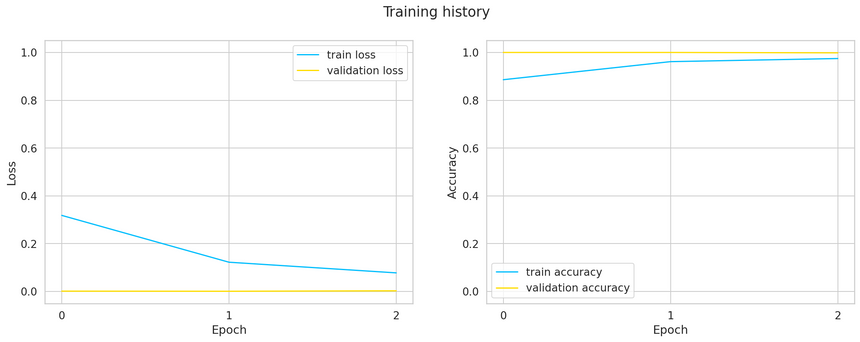

The pre-trained model is so good that we get very high accuracy and low loss after 3 epochs. Unfortunately, our validation set is too small to get some meaningful metrics from it.

Evaluation

Let’s see some predictions on traffic signs from the test set:

1def show_predictions(model, class_names, n_images=6):
2  model = model.eval()
3  images_handeled = 0
4  plt.figure()
5
6  with torch.no_grad():
7    for i, (inputs, labels) in enumerate(data_loaders['test']):
8      inputs = inputs.to(device)
9      labels = labels.to(device)
10
11      outputs = model(inputs)
12      _, preds = torch.max(outputs, 1)
13
14      for j in range(inputs.shape[0]):
15        images_handeled += 1
16        ax = plt.subplot(2, n_images//2, images_handeled)
17        ax.set_title(f'predicted: {class_names[preds[j]]}')
18        imshow(inputs.cpu().data[j])
19        ax.axis('off')
20
21        if images_handeled == n_images:
22          return

1show_predictions(base_model, class_names, n_images=8)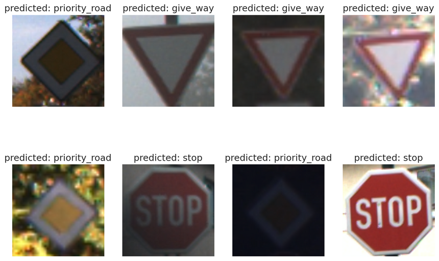

Very good! Even the almost not visible priority road sign is classified correctly. Let’s dive a bit deeper.

We’ll start by getting the predictions from our model:

1def get_predictions(model, data_loader):
2  model = model.eval()
3  predictions = []
4  real_values = []
5  with torch.no_grad():
6    for inputs, labels in data_loader:
7      inputs = inputs.to(device)
8      labels = labels.to(device)
9
10      outputs = model(inputs)
11      _, preds = torch.max(outputs, 1)
12      predictions.extend(preds)
13      real_values.extend(labels)
14  predictions = torch.as_tensor(predictions).cpu()
15  real_values = torch.as_tensor(real_values).cpu()
16  return predictions, real_values

1y_pred, y_test = get_predictions(base_model, data_loaders['test'])

1print(classification_report(y_test, y_pred, target_names=class_names))

1precision    recall  f1-score   support
2
3         give_way       1.00      1.00      1.00       216
4         no_entry       1.00      1.00      1.00       111
5    priority_road       1.00      1.00      1.00       210
6             stop       1.00      1.00      1.00        78
7
8         accuracy                           1.00       615
9        macro avg       1.00      1.00      1.00       615
10     weighted avg       1.00      1.00      1.00       615

The classification report shows us that our model is perfect, not something you see every day! Does this thing make any mistakes?

1def show_confusion_matrix(confusion_matrix, class_names):
2
3  cm = confusion_matrix.copy()
4
5  cell_counts = cm.flatten()
6
7  cm_row_norm = cm / cm.sum(axis=1)[:, np.newaxis]
8
9  row_percentages = ["{0:.2f}".format(value) for value in cm_row_norm.flatten()]
10
11  cell_labels = [f"{cnt}\n{per}" for cnt, per in zip(cell_counts, row_percentages)]
12  cell_labels = np.asarray(cell_labels).reshape(cm.shape[0], cm.shape[1])
13
14  df_cm = pd.DataFrame(cm_row_norm, index=class_names, columns=class_names)
15
16  hmap = sns.heatmap(df_cm, annot=cell_labels, fmt="", cmap="Blues")
17  hmap.yaxis.set_ticklabels(hmap.yaxis.get_ticklabels(), rotation=0, ha='right')
18  hmap.xaxis.set_ticklabels(hmap.xaxis.get_ticklabels(), rotation=30, ha='right')
19  plt.ylabel('True Sign')
20  plt.xlabel('Predicted Sign');

1cm = confusion_matrix(y_test, y_pred)
2show_confusion_matrix(cm, class_names)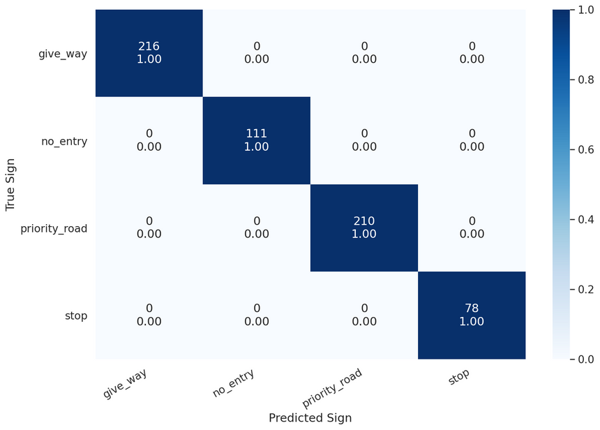

No, no mistakes here!

Classifying unseen images

Ok, but how good our model will be when confronted with a real-world image? Let’s check it out:

1!gdown --id 19Qz3a61Ou_QSHsLeTznx8LtDBu4tbqHr

1show_image('stop-sign.jpg')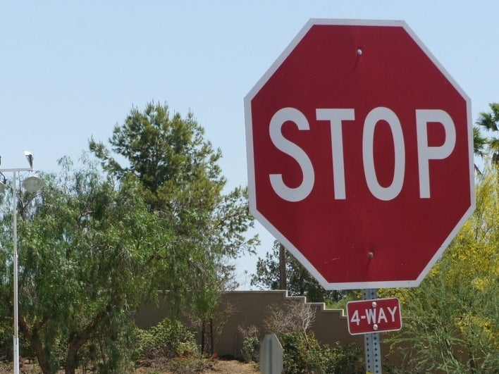

For this, we’ll have a look at the confidence for each class. Let’s get this from our model:

1def predict_proba(model, image_path):
2  img = Image.open(image_path)
3  img = img.convert('RGB')
4  img = transforms['test'](img).unsqueeze(0)
5
6  pred = model(img.to(device))
7  pred = F.softmax(pred, dim=1)
8  return pred.detach().cpu().numpy().flatten()

1pred = predict_proba(base_model, 'stop-sign.jpg')
2pred

1array([1.1296713e-03, 1.9811286e-04, 3.4486805e-04, 9.9832731e-01],
2          dtype=float32)

This is a bit hard to understand. Let’s plot it:

1def show_prediction_confidence(prediction, class_names):
2  pred_df = pd.DataFrame({
3    'class_names': class_names,
4    'values': prediction
5  })
6  sns.barplot(x='values', y='class_names', data=pred_df, orient='h')
7  plt.xlim([0, 1]);

1show_prediction_confidence(pred, class_names)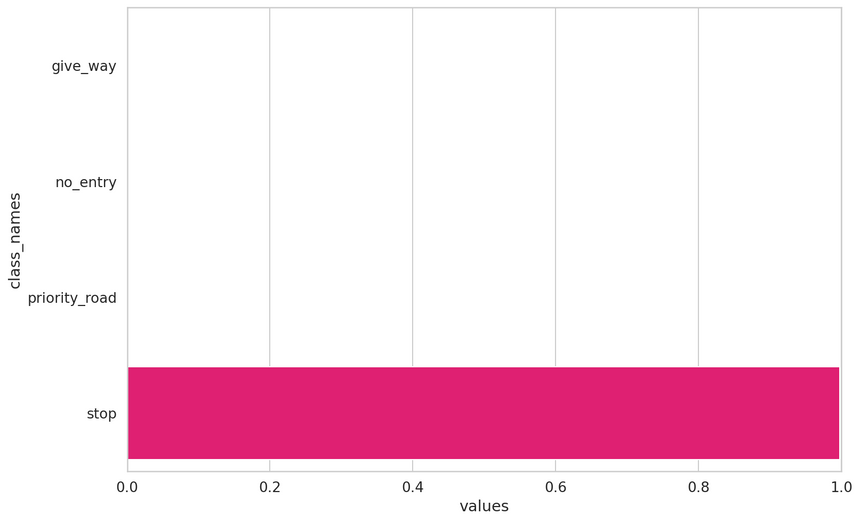

Again, our model is performing very well! Really confident in the correct traffic sign!

Classyfing unknown traffic sign

The last challenge for our model is a traffic sign that it hasn’t seen before:

1!gdown --id 1F61-iNhlJk-yKZRGcu6S9P29HxDFxF0u

1show_image('unknown-sign.jpg')

Let’s get the predictions:

1pred = predict_proba(base_model, 'unknown-sign.jpg')
2pred

1array([9.9413127e-01, 1.1861280e-06, 3.9936006e-03, 1.8739274e-03],
2          dtype=float32)

1show_prediction_confidence(pred, class_names)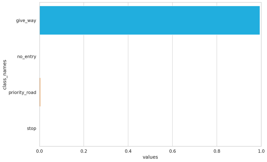

Our model is very certain (more than 95% confidence) that this is a give way sign. This is obviously wrong. How can you make your model see this?

Adding class “unknown”

While there are a variety of ways to handle this situation (one described in this paper: A Baseline for Detecting Misclassified and Out-of-Distribution Examples in Neural Networks), we’ll do something simpler.

We’ll get the indices of all traffic signs that weren’t included in our original dataset:

1unknown_indices = [
2  i for i, f in enumerate(train_folders) \
3  if i not in class_indices
4]
5
6len(unknown_indices)

We’ll create a new folder for the unknown class and copy some of the images there:

1for ds in DATASETS:
2  (DATA_DIR / ds / 'unknown').mkdir(parents=True, exist_ok=True)
3
4for ui in unknown_indices:
5  image_paths = np.array(glob(f'{train_folders[ui]}/*.ppm'))
6  image_paths = np.random.choice(image_paths, 50)
7
8  ds_split = np.split(
9    image_paths,
10    indices_or_sections=[int(.8*len(image_paths)), int(.9*len(image_paths))]
11  )
12
13  dataset_data = zip(DATASETS, ds_split)
14
15  for ds, images in dataset_data:
16    for img_path in images:
17      shutil.copy(img_path, f'{DATA_DIR}/{ds}/unknown/')

The next steps are identical to what we’ve already done:

1image_datasets = {
2  d: ImageFolder(f'{DATA_DIR}/{d}', transforms[d]) for d in DATASETS
3}
4
5data_loaders = {
6  d: DataLoader(image_datasets[d], batch_size=4, shuffle=True, num_workers=4)
7  for d in DATASETS
8}
9
10dataset_sizes = {d: len(image_datasets[d]) for d in DATASETS}
11class_names = image_datasets['train'].classes
12
13dataset_sizes

1{'test': 784, 'train': 5704, 'val': 794}

1%%time
2
3enchanced_model = create_model(len(class_names))
4enchanced_model, history = train_model(enchanced_model, data_loaders, dataset_sizes, device)

1Epoch 1/3
2    ----------
3    Train loss 0.39523224640235327 accuracy 0.8650070126227208
4    Val   loss 0.002290595416447625 accuracy 1.0
5
6    Epoch 2/3
7    ----------
8    Train loss 0.173455789528505 accuracy 0.9446002805049089
9    Val   loss 0.030148923471944415 accuracy 0.9886649874055415
10
11    Epoch 3/3
12    ----------
13    Train loss 0.11575758963990512 accuracy 0.9640603085553997
14    Val   loss 0.0014996432778823317 accuracy 1.0
15
16    Best val accuracy: 1.0
17    CPU times: user 2min 47s, sys: 56.2 s, total: 3min 44s
18    Wall time: 3min 53s

1plot_training_history(history)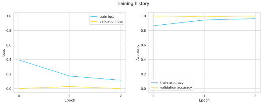

Again, our model is learning very quickly. Let’s have a look at the sample image again:

1show_image('unknown-sign.jpg')

1pred = predict_proba(enchanced_model, 'unknown-sign.jpg')
2show_prediction_confidence(pred, class_names)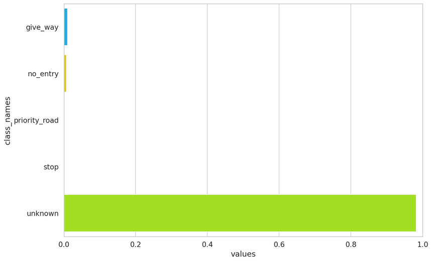

Great, the model doesn’t give much weight to any of the known classes. It doesn’t magically know that this is a two-way sign, but recognizes is as unknown.

Let’s have a look at some examples of our new dataset:

1show_predictions(enchanced_model, class_names, n_images=8)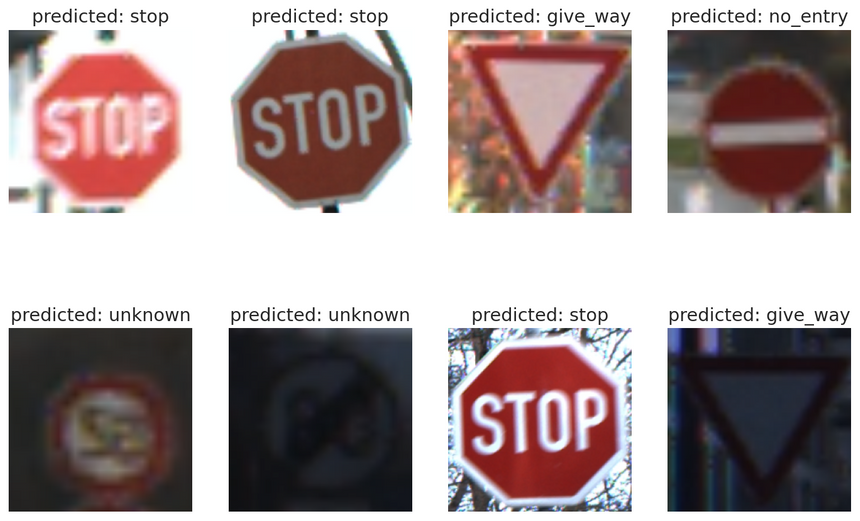

Let’s get an overview of the new model’s performance:

1y_pred, y_test = get_predictions(enchanced_model, data_loaders['test'])

1print(classification_report(y_test, y_pred, target_names=class_names))

1precision    recall  f1-score   support
2
3         give_way       1.00      1.00      1.00       216
4         no_entry       1.00      1.00      1.00       111
5    priority_road       1.00      1.00      1.00       210
6             stop       1.00      1.00      1.00        78
7          unknown       1.00      1.00      1.00       169
8
9         accuracy                           1.00       784
10        macro avg       1.00      1.00      1.00       784
11     weighted avg       1.00      1.00      1.00       784

1cm = confusion_matrix(y_test, y_pred)
2show_confusion_matrix(cm, class_names)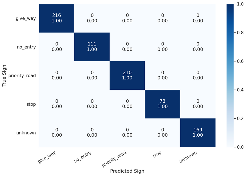

Our model is still perfect. Go ahead, try it on more images!

Summary

Good job! You trained two different models for classifying traffic signs from raw pixels. You also built a dataset that is compatible with Torchvision.

Here’s what you’ve learned:

Overview of the traffic sign image dataset
Build a dataset
Use a pre-trained model from Torchvision
Add a new unknown class and re-train the model

Can you use transfer learning for other tasks? How do you do it? Let me know in the comments below.

References

Want to be a Machine Learning expert?

Join the weekly newsletter on Data Science, Deep Learning and Machine Learning in your inbox, curated by me! Chosen by 10,000+ Machine Learning practitioners. (There might be some exclusive content, too!)

You'll never get spam from me

Hacker's Guide to Neural Networks in JavaScript

Build Machine Learning models (especially Deep Neural Networks) that you can easily integrate with existing or new web apps. Think of your ReactJs, Vue, or Angular app enhanced with the power of Machine Learning models.

Get SH*T Done with PyTorch

Learn how to solve real-world problems with Deep Learning models (NLP, Computer Vision, and Time Series). Go from prototyping to deployment with PyTorch and Python!

Hacker's Guide to Machine Learning with Python

This book brings the fundamentals of Machine Learning to you, using tools and techniques used to solve real-world problems in Computer Vision, Natural Language Processing, and Time Series analysis. The skills taught in this book will lay the foundation for you to advance your journey to Machine Learning Mastery!

Hands-On Machine Learning from Scratch

This book will guide you on your journey to deeper Machine Learning understanding by developing algorithms in Python from scratch! Learn why and when Machine learning is the right tool for the job and how to improve low performing models!